Section 10 Abundance vs. vocalization rates
In this script, we model correlations between abundance (as estimated via point count data) and vocalization rates (calculated from acoustic data).
10.3 Estimate abundance from point count data and calculate vocalization rates from acoustic data
Here, we make a distinction before running correlative analyses that abundance corresponds to the total number of individuals of a species detected across visits to a site and can only be calculated for point count data.
Unlike the previous script, where we used a measure of detections from the acoustic data, we will calculate a measure which we define as vocalization rates. Vocalization rate is calculated as the number of vocalizations (detections across 10-s clips) for a particular time period. Here, time period is defined as the number of total number of 10s-clips across the number of visits to that site. In other words, each site can have ~4 to 5 16-min acoustic surveys at that site.
The total number of acoustic detections for a single acoustic survey can range from 0 to 96, where 96 corresponds to the number of 10-s clips that were analyzed across the 16-min window. If there were 4 or 5 visits to a site, this number can range from 0 to (384/480) [in other words, 96x4 or 96x5].
Hence, the vocalization rate for each species at a site is defined as (x number of vocalizations)/(total number of 10-s clips analyzed). The total number of 10-s clips analyzed can vary depending on the number of visits to the site.
# point-count data
# estimate total abundance of all species for each site
abundance <- datSubset %>%
  filter(data_type == "point_count") %>%
  group_by(site_id, restoration_type, scientific_name,
           common_name, eBird_codes) %>%
  summarise(abundance_pc = sum(number)) %>%
  ungroup()

# for acoustic data, we will first estimate the number of visits to a site, which will essentially translate to the number of 10-s clips that were analyzed/heard (used here as the time period for the calculation of vocalization rates)

# nVisits is calculated here
# except for INBS04U, all other sites had a total of 5 visits, while INBS04U had 4 visits
nSitesDays <- datSubset %>%
  filter(data_type == "acoustic_data") %>%
  dplyr::select(site_id, date)%>%
  distinct() %>% arrange(site_id) %>% count(site_id) %>%
  rename(nVisits = n)

# estimate total number of detections across the acoustic data
# note: we cannot call this abundance as it refers to the total number of vocalizations across all sites
detections <- datSubset %>%
  filter(data_type == "acoustic_data") %>%
  group_by(site_id, restoration_type, scientific_name,
           common_name, eBird_codes) %>%
  summarise(detections_aru = sum(number)) %>%
  ungroup()

# estimating vocalization rates for each species for each site
vocRate <- detections %>%
  left_join(., nSitesDays, by = "site_id") %>%
  mutate(nClips = nVisits*96) %>%
  mutate(vocRate = detections_aru/nClips)

# Note that the column vocRate can vary between 0 to 1 for each species for each site (this value can vary across sites for each species, referring to how vocally active a species is)
10.4 Correlations between abundance and vocalization rates
# create a single dataframe
data <- full_join(abundance, vocRate)%>%
  replace_na(list(abundance_pc = 0, detections_aru = 0,
                  nVisits = 0, nClips = 0, vocRate = 0))

# only those species that have a minimum abundance value of 10 and minimum detection value of 10
spp_subset <-  data %>%
  group_by(scientific_name) %>%
  summarise(abundance_pc = sum(abundance_pc), detections_aru = sum(detections_aru)) %>%
  ungroup() %>%
  filter(abundance_pc >=10 & detections_aru >= 10)

# subset data
data <- data %>%
  filter(scientific_name %in% spp_subset$scientific_name)

# reordering factors for plotting
data$restoration_type <- factor(data$restoration_type, levels = c("BM", "AR", "NR"))

# visualization
fig_abund_vocRate_cor <- grouped_ggscatterstats(
  data = data,
  x = vocRate,
  y = abundance_pc,
  grouping.var = restoration_type,
  type = "r",
  plotgrid.args = list(nrow = 3, ncol = 1),
  ggplot.component = list(theme(text = element_text(family = "Century Gothic", size = 15, face = "bold"),plot.title = element_text(family = "Century Gothic",
      size = 18, face = "bold"),
      plot.subtitle = element_text(family = "Century Gothic",
      size = 15, face = "bold",color="#1b2838"),
      axis.title = element_text(family = "Century Gothic",
      size = 15, face = "bold"))))

ggsave(fig_abund_vocRate_cor, filename = "figs/fig_abundance_vs_vocRates_correlations.png", width = 14, height = 16, device = png(), units = "in", dpi = 300)
dev.off() 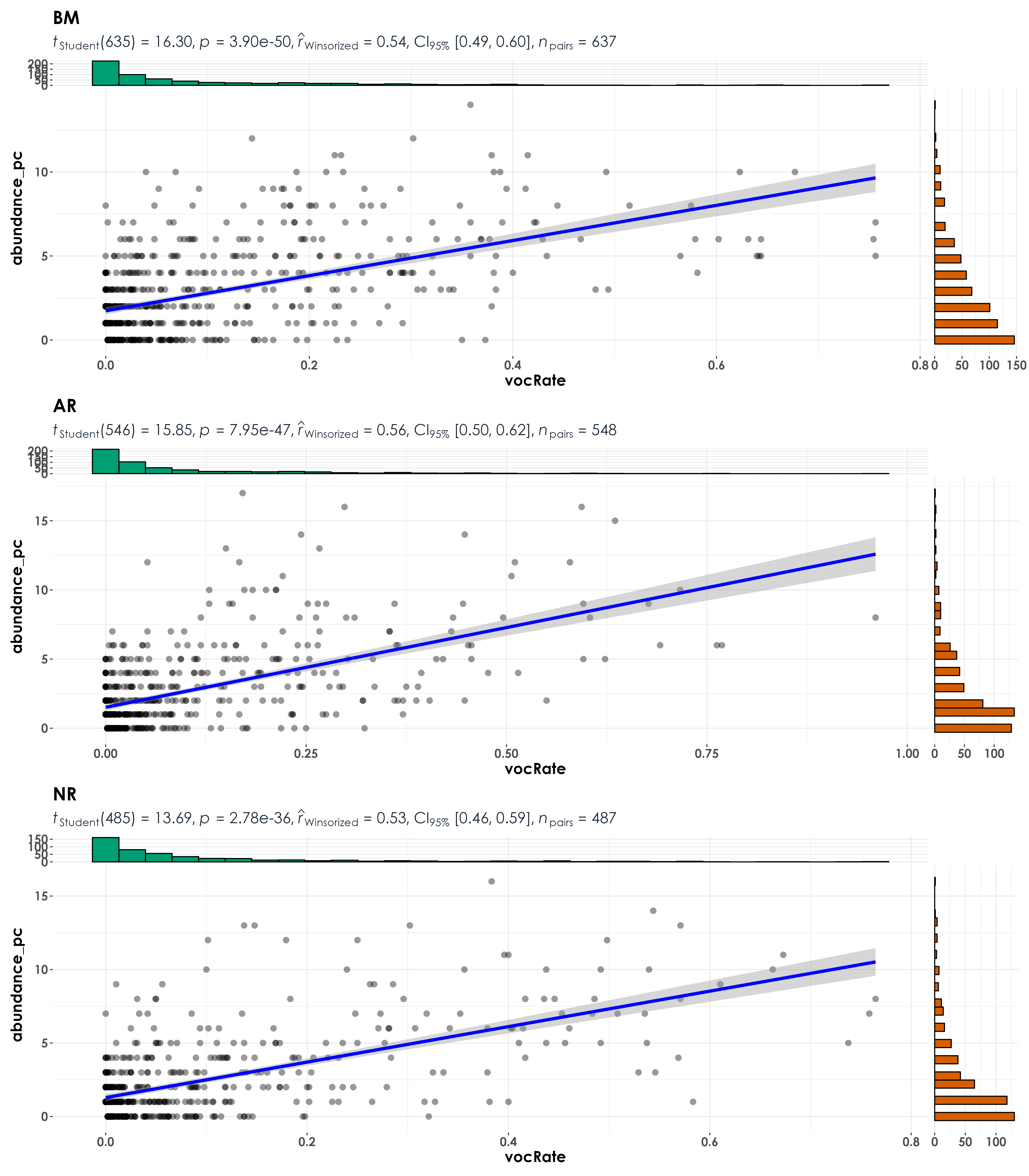
10.5 Regressions between abundance and vocalization rates
data <- setDT(data)
# extract t-value
data[, t_value := summary(lm(vocRate ~ abundance_pc))$coefficients[6], by = scientific_name]
# extract slope
data[, slope := lm(vocRate ~ abundance_pc)%>% coef()%>% nth(2), by = scientific_name]
# extract pearson's correlation
data[, pearson := cor(vocRate, abundance_pc), by = scientific_name]
# extract adjusted r squared
data[, r_sq := summary(lm(vocRate ~ abundance_pc))$adj.r.squared, by = scientific_name]
# create a column with the direction of the slope (whether it is positive or negative), which can be referred to later while plotting
data[, slope_dir := ifelse(slope >0, '+', '-')]
paste("Positive regressions:",length(unique(data$scientific_name[data$slope_dir %in% c('+')])))
# 39 species had a positive regression or slope value
## visualization
fig_abund_vocRate_reg <- ggplot(data, aes(y = vocRate,
x = abundance_pc)) +
geom_point(color = "#9CC3D5",size = 1.2) +
geom_smooth(data = data, aes(group = scientific_name,
color = slope_dir),
method = 'lm', se = FALSE,
linewidth = 0.7) +
scale_color_manual(values=c("#1B9E77", "#D95F02")) +
labs(y="\nVocalization rate (from acoustic data)",
x="Abundance (from point count data)\n") +
theme_bw() +
annotate("text", x=13, y=0.9,
label= "Slope:", col = "grey30", size = 12) +
annotate("text", x=16, y=0.9,
label= "+", col = "#D95F02", size = 12) +
annotate("text", x = 18, y=0.9,
label = "-", col = "#1B9E77", size = 12)+
theme(text = element_text(family = "Century Gothic", size = 18, face = "bold"),plot.title = element_text(family = "Century Gothic",
size = 18, face = "bold"),
plot.subtitle = element_text(family = "Century Gothic",
size = 15, face = "bold",color="#1b2838"),
axis.title = element_text(family = "Century Gothic",
size = 18, face = "bold"),
legend.position = "none")
ggsave(fig_abund_vocRate_reg, filename = "figs/fig_abundance_vs_vocRates_regressions.png", width = 14, height = 16, device = png(), units = "in", dpi = 300)
dev.off()
# extract the slope, t_value, pearson correlation and the adjusted r square
lm_output <- data %>%
dplyr::select(scientific_name, t_value, slope, pearson, slope_dir,r_sq) %>% distinct()
# write the values to file
write.csv(lm_output, "results/abundance-vocRates-regressions.csv",
row.names = F)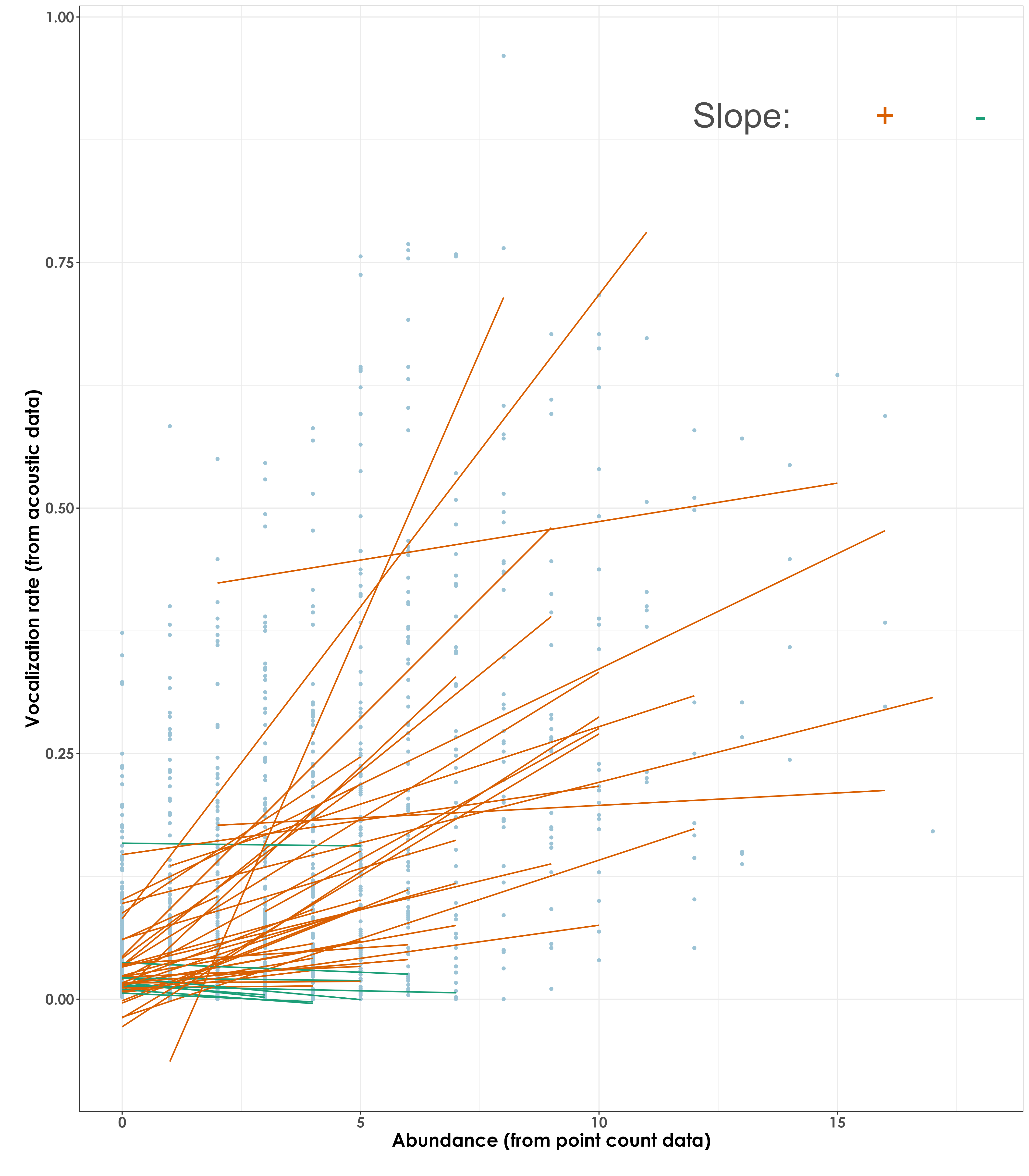 ## Plotting species-specific regression plots
# visualization
plots <- list()
for(i in 1:length(unique(data$scientific_name))){
# extract species scientific name
a <- unique(data$scientific_name)[i]
# subset data for plotting
for_plot <- data[data$scientific_name==a,]
# create plots
plots[[i]] <- ggplot(for_plot, aes(y = vocRate,
x = abundance_pc)) +
geom_point(color = "#9CC3D5",size = 1.2) +
geom_smooth(aes(color = "#D95F02"),
method = 'lm', se = TRUE,
linewidth = 0.7) +
labs(title = paste0(a," ","r_sq = ", signif(for_plot$r_sq, digits = 2), " ", paste0("slope = ",signif(for_plot$slope, digits = 4))),
y="\nVocalization rates (from acoustic data)",
x="Abundance (from point count data)\n") +
theme_bw() +
theme(text = element_text(family = "Century Gothic", size = 18, face = "bold"),plot.title = element_text(family = "Century Gothic",
size = 18, face = "bold"),
plot.subtitle = element_text(family = "Century Gothic",
size = 15, face = "bold",color="#1b2838"),
axis.title = element_text(family = "Century Gothic",
size = 18, face = "bold"),
legend.position = "none")
}
# plot and save as a single pdf
cairo_pdf(
filename = "figs/abundance-vocRates-by-species-regressions.pdf",
width = 13, height = 12,
onefile = TRUE
)
plots
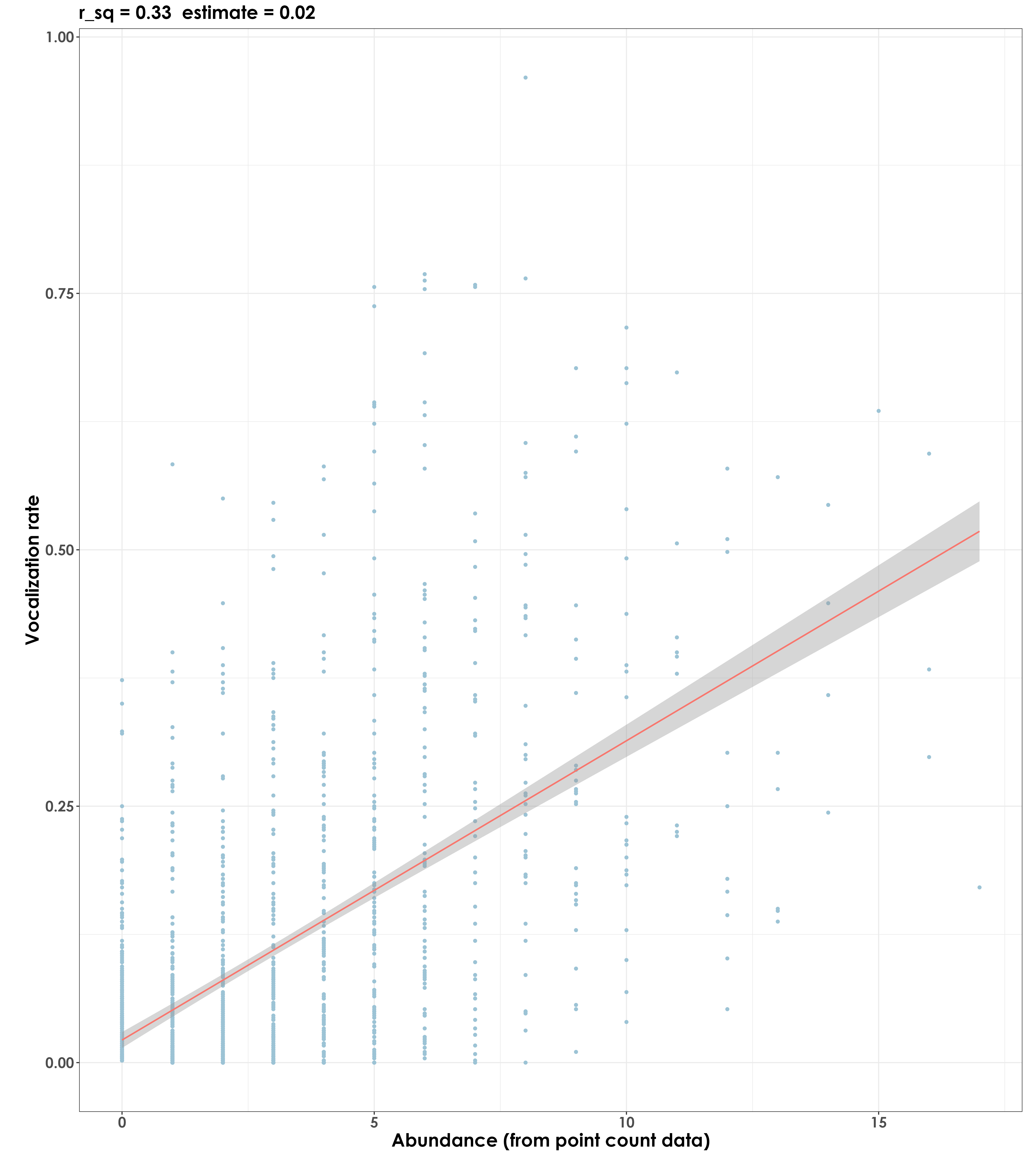
dev.off() 10.6 Community-level regressions
In this visualization, we essentially plot overall data of acoustic detections against abundance (from point count data)
comm_reg <- lm(vocRate ~ abundance_pc, data=data)
summary(comm_reg)

# Call:
# lm(formula = vocRate ~ abundance_pc, data = data)

# Residuals:
#     Min       1Q   Median       3Q      Max
# -0.34720 -0.06162 -0.01993  0.03007  0.70498

# Coefficients:
#             Estimate Std. Error t value Pr(>|t|)
# (Intercept)  0.022013   0.003962   5.555 3.22e-08 ***
# abundance_pc 0.029178   0.001018  28.674  < 2e-16 ***

# Residual standard error: 0.1185 on 1670 degrees of freedom
# Multiple R-squared:  0.3299,  Adjusted R-squared:  0.3295
# F-statistic: 822.2 on 1 and 1670 DF,  p-value: < 2.2e-16

# visualization
fig_abund_vocRate_comm_reg <- ggplot(data, aes(y = vocRate,x = abundance_pc)) +
  geom_point(color = "#9CC3D5",size = 1.2) +
  geom_smooth(aes(color = "#D95F02"),
    method = 'lm', se = TRUE,
              linewidth = 0.7) +
    labs(title = paste0("r_sq = 0.33", "  ", paste0("estimate = 0.02")),
      y="\nVocalization rate",
       x="Abundance (from point count data)\n") +
    theme_bw() +
  theme(text = element_text(family = "Century Gothic", size = 18, face = "bold"),plot.title = element_text(family = "Century Gothic",
      size = 18, face = "bold"),
      plot.subtitle = element_text(family = "Century Gothic",
      size = 15, face = "bold",color="#1b2838"),
      axis.title = element_text(family = "Century Gothic",
      size = 18, face = "bold"),
      legend.position = "none")

ggsave(fig_abund_vocRate_comm_reg, filename = "figs/fig_abundance_vs_vocRates_regressions_communityLevel.png", width = 14, height = 16, device = png(), units = "in", dpi = 300)
dev.off()