Section 13 Body mass
In this script, we will explore relationships between the ratio of bird detections in a point count and acoustic survey and the body mass of a species. To do this, we will continue to rely on detections estimated at the site-level (similar to what was required for the indicator species analysis).
To get at this measure, we estimate detections at the site level (for a total of six visits). If the across_visit_detections = 6, that means that a species was detected every single time across each of the six visits to that site. This value ranges from 1 to 6 for each species for a point count and acoustic survey.
13.1 Load necessary libraries
library(tidyverse)
library(dplyr)
library(stringr)
library(vegan)
library(ggplot2)
library(scico)
library(psych)
library(ecodist)
library(RColorBrewer)
library(ggforce)
library(ggalt)
library(patchwork)
library(sjPlot)
library(ggside)
library(ggstatsplot)
library(extrafont)
library(scales)

# Source any custom/other internal functions necessary for analysis
source("code/01_internal-functions.R")13.4 Visit-level detection estimates for each species
We estimate the total number of detections of each species across all visits. This can vary between 1 and 6 for point counts (since a total of six visits were made to each site), while this number can vary between 1 to 5 for acoustic surveys. To account for the slight difference in the number of visits, we scale the data to go between 1 and 10 (arbitrarily chosen) to ensure that the visit-level estimates are comparable.
## we will estimate abundance across point counts by site-date (essentially corresponding to visit)
abundance <- datSubset %>%
  filter(data_type == "point_count") %>%
  group_by(date, site_id, restoration_type, scientific_name,
           common_name, eBird_codes) %>%
  summarise(totAbundance = sum(number)) %>%
  ungroup()

# estimate across visit detections for point count data
pc_visit_detections <- abundance %>%
  mutate(forDetections = case_when(totAbundance > 0 ~ 1)) %>%
  group_by(scientific_name, site_id,restoration_type) %>%
  summarise(pc_visit_detections = sum(forDetections)) %>%
  mutate(data_type = "point_count") %>%
  ungroup()

# scale values to go between 1 and 10
pc_visit_detections$pc_visit_scaled <- rescale(pc_visit_detections$pc_visit_detections, to = c(1,10))

# estimate total number of detections across the acoustic data by site-date (essentially corresponds to a visit)
# note: we cannot call this abundance as it refers to the total number of vocalizations across a 16-min period across all sites
detections <- datSubset %>%
  filter(data_type == "acoustic_data") %>%
  group_by(date, site_id, restoration_type, scientific_name,
           common_name, eBird_codes) %>%
  summarise(totDetections = sum(number)) %>%
  ungroup()

# estimate across visit detections for acoustic data
aru_visit_detections <- detections %>%
  mutate(forDetections = case_when(totDetections > 0 ~ 1)) %>%
  group_by(scientific_name, site_id,restoration_type) %>%
  summarise(aru_visit_detections = sum(forDetections)) %>%
  mutate(data_type = "acoustic_data") %>%
  ungroup()

# scale values to go between 1 and 10
aru_visit_detections$aru_visit_scaled <- rescale(aru_visit_detections$aru_visit_detections, to = c(1,10))
13.5 Exploring ratios of detections in point counts & acoustic surveys to body mass of a species
# create a single dataframe
visit_detections <- full_join(pc_visit_detections[,-5], aru_visit_detections[,-5]) %>%
replace_na(list(pc_visit_detections = 0, aru_visit_detections = 0,
pc_visit_scaled = 0, aru_visit_scaled = 0))
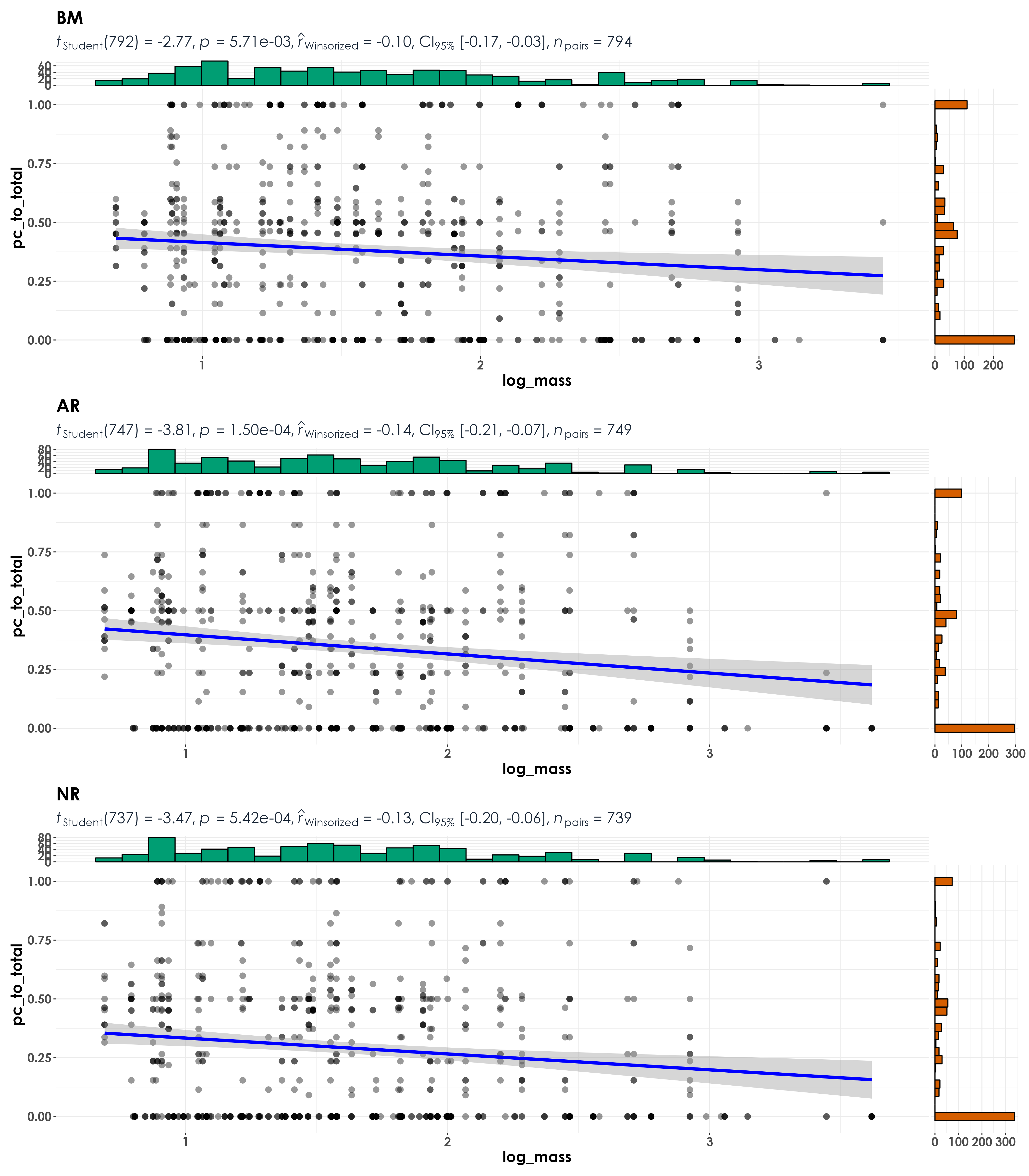
# create column of ratio of detections of point counts to total number of detections from point count and acoustic data
# note: if there are no detections through the acoustic survey, the ratio will be 1; if there are equal number of detections in the acoustic survey and point count data, the ratio will be 0.5; if there no detections/lesser detections in a point count compared to acoustic survey, the ratio will be between 0 and 0.5; and lastly, if there are more detections in a point count compared to an acoustic survey, the ratio will be between 0.5 and 1.
visit_detections <- visit_detections %>%
mutate(pc_to_total = (pc_visit_scaled)/
(pc_visit_scaled + aru_visit_scaled))
# add species trait data i.e. body mass to the above dataframe
visit_detections <- left_join(visit_detections,
trait[,c(1,26)], by = "scientific_name")
# log-transform body mass
visit_detections$log_mass <- log10(visit_detections$mass)
# reordering factors for plotting
visit_detections$restoration_type <- factor(visit_detections$restoration_type, levels = c("BM", "AR", "NR"))
# visualization
fig_bodyMass <- grouped_ggscatterstats(
data = visit_detections,
x = log_mass,
y = pc_to_total,
grouping.var = restoration_type,
type = "r",
plotgrid.args = list(nrow = 3, ncol = 1),
ggplot.component = list(theme(text = element_text(family = "Century Gothic", size = 15, face = "bold"),plot.title = element_text(family = "Century Gothic",
size = 18, face = "bold"),
plot.subtitle = element_text(family = "Century Gothic",
size = 15, face = "bold",color="#1b2838"),
axis.title = element_text(family = "Century Gothic",
size = 15, face = "bold"))))
ggsave(fig_bodyMass, filename = "figs/fig_bodyMass_detectionRatio_correlations.png", width = 14, height = 16, device = png(), units = "in", dpi = 300)
dev.off()