Section 3 Richness estimates
In this script, we will calculate species richness estimates across point count surveys and acoustic data. We estimate differences in species richness by habitat affiliation and foraging guilds.
3.4 Estimate richness for point count and acoustic data
# point-count data
# estimate total abundance across all species for each site
abundance <- datSubset %>%
  filter(data_type == "point_count") %>%
  group_by(site_id, scientific_name,
           common_name, eBird_codes, habitat, foraging_habit) %>% summarise(totAbundance = sum(number)) %>%
  ungroup()

# total abundance by species
pc_totAbundance <- abundance %>%
  group_by(scientific_name, common_name, habitat, foraging_habit) %>%
  summarise(totAbundance = sum(totAbundance))

# species most abundant in a point count include the Nilgiri flowerpecker, Greenish Warbler, White-cheeked Barbet, Yellow-browed Bulbul, Vernal-hanging Parrot

# estimate richness for point count data (calculated for each site)
pc_richness <- abundance %>%
  mutate(forRichness = case_when(totAbundance > 0 ~ 1)) %>%
  group_by(site_id) %>%
  summarise(richness = sum(forRichness)) %>%
  mutate(data_type = "point_count") %>%
  ungroup()

# estimate total number of detections across the acoustic data
# note: we cannot call this abundance as it refers to the total number of vocalizations across a 15-min period across all sites
detections <- datSubset %>%
  filter(data_type == "acoustic_data") %>%
  group_by(site_id, scientific_name,
           common_name, eBird_codes, habitat, foraging_habit) %>% summarise(totDetections = sum(number)) %>%
  ungroup()

# total number of detections by species
aru_totDetections <- detections %>%
  group_by(scientific_name, common_name, habitat, foraging_habit) %>%
  summarise(totDetections = sum(totDetections))

# species with the highest numbers of acoustic detections across sites are the White-cheeked Barbet, Crimson-backed Sunbird, Nilgiri Flowerpecker, Red-whiskered Bulbul and Greenish Warbler

# estimate richness for acoustic data
aru_richness <- detections %>%
  mutate(forRichness = case_when(totDetections > 0 ~ 1)) %>%
  group_by(site_id) %>%
  summarise(richness = sum(forRichness)) %>%
  mutate(data_type = "acoustic_data") %>%
  ungroup()

# how many species were detected in a point count but not acoustic data?
# four species were detected that were not observed in acoustic surveys
pc_not_aru <- anti_join(pc_totAbundance, aru_totDetections)
write.csv(pc_not_aru, "results/species-in-pointCount-not-acoustics.csv", row.names = F)

# how many species were detected in acoustic data but not point counts?
# 31 species were detected in acoustic data, but not in point counts
aru_not_pc <- anti_join(aru_totDetections, pc_totAbundance)
write.csv(aru_not_pc, "results/species-in-acoustics-not-pointCounts.csv", row.names = F)
3.5 Visualize differences in richness between point count data and acoustic data
richness <- bind_rows(pc_richness, aru_richness)

# Here, we use functions from the package ggstatsplot (more information can be found here:https://indrajeetpatil.github.io/ggstatsplot/index.html)

fig_richness <- richness %>%
  ggbetweenstats(x = data_type,
                         y = richness,
                         xlab = "Data type",
                         ylab = "Richness",
                         pairwise.display = "significant",
                         package = "ggsci",
                         palette = "default_jco",
    plotgrid.args = list(nrow = 3),
ggplot.component = list(theme(text = element_text(family = "Century Gothic", size = 15, face = "bold"),plot.title = element_text(family = "Century Gothic",
      size = 18, face = "bold"),
      plot.subtitle = element_text(family = "Century Gothic",
      size = 15, face = "bold",color="#1b2838"),
      axis.title = element_text(family = "Century Gothic",
      size = 15, face = "bold"))))

ggsave(fig_richness, filename = "figs/fig_richness.png", width = 13, height = 14, device = png(), units = "in", dpi = 300)
dev.off() 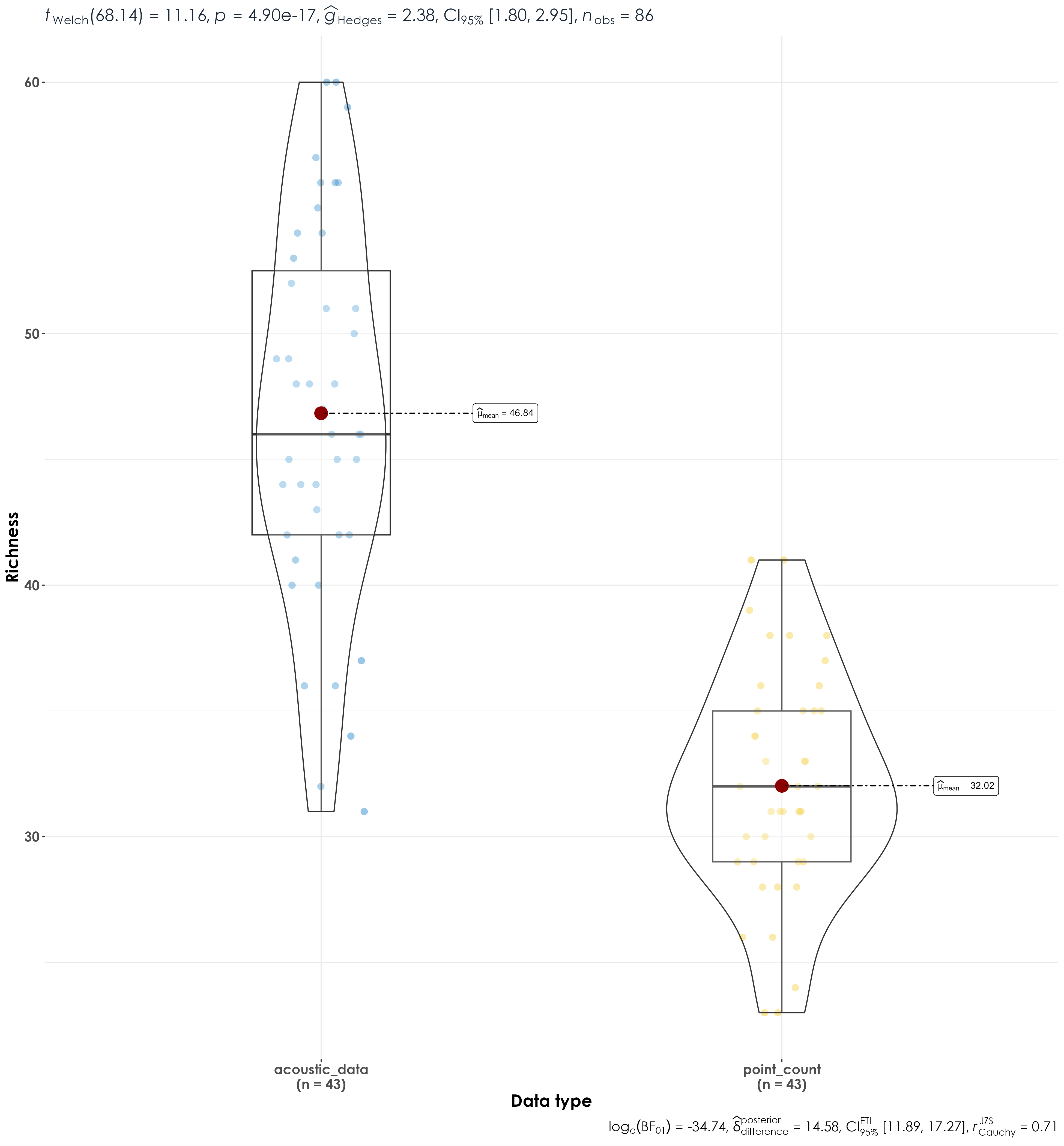
Significant differences in richness between acoustic data and point count data.
3.6 Visualize differences in richness as a function of species habitat affiliation
Here, we examine if there are differences in species richness between point counts and acoustic surveys as a function of habitat affiliation - whether a species is a rainforest specialist or an open-country generalists.
# estimate richness by trait for point count data
trait_pc_richness <- abundance %>%
  mutate(forRichness = case_when(totAbundance > 0 ~ 1)) %>%
  group_by(site_id, habitat) %>%
  summarise(richness = sum(forRichness)) %>%
  mutate(data_type = "point_count") %>%
  ungroup()

# estimate richness by trait for acoustic data
trait_aru_richness <- detections %>%
  mutate(forRichness = case_when(totDetections > 0 ~ 1)) %>%
  group_by(site_id, habitat) %>%
  summarise(richness = sum(forRichness)) %>%
  mutate(data_type = "acoustic_data") %>%
  ungroup()

# bind rows prior to visualization
trait_richness <- bind_rows(trait_pc_richness, trait_aru_richness)

# visualization
fig_trait_richness <- trait_richness %>%
  grouped_ggbetweenstats(x = data_type,
                         y = richness,
                         grouping.var = habitat,
                         xlab = "Data type",
                         ylab = "Richness",
                         pairwise.display = "significant",
                         package = "ggsci",
                         palette = "default_jco",
ggplot.component = list(theme(text = element_text(family = "Century Gothic", size = 15, face = "bold"),plot.title = element_text(family = "Century Gothic",
      size = 18, face = "bold"),
      plot.subtitle = element_text(family = "Century Gothic",
      size = 15, face = "bold",color="#1b2838"),
      axis.title = element_text(family = "Century Gothic",
      size = 15, face = "bold"))))

ggsave(fig_trait_richness, filename = "figs/fig_richness_by_trait.png", width = 13, height = 14, device = png(), units = "in", dpi = 300)
dev.off() 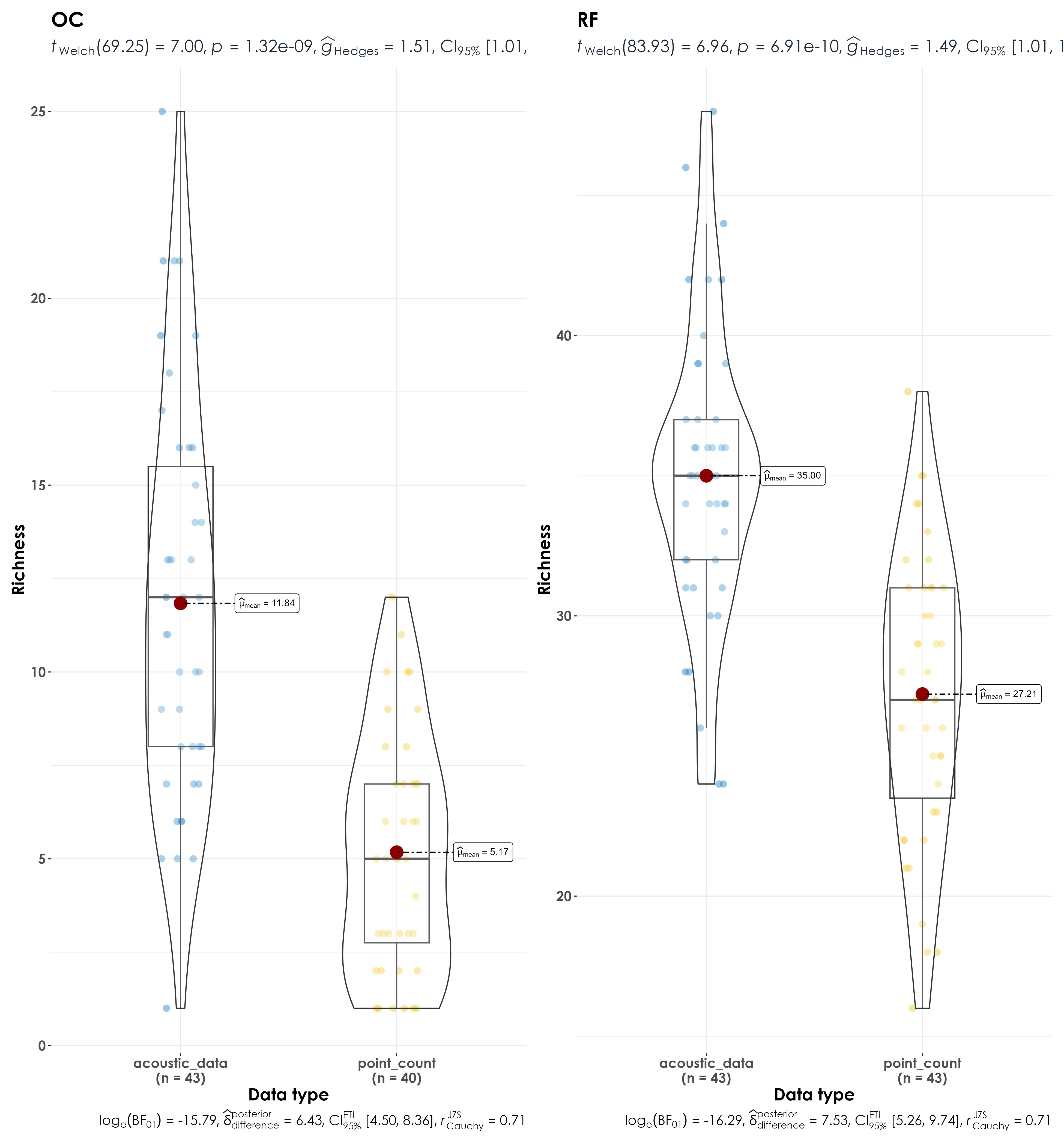
Significant differences in richness of birds between acoustic data and point count data as a function of species trait
3.7 Visualize differences in species richness as a function of species foraging guilds
Here, we examine if there are differences in species richness between point counts and acoustic surveys as a function of foraging guilds - whether a species forages on the ground, understorey, mid-storey, or canopy.
# estimate richness by foraging habit for point count data
foraging_pc_richness <- abundance %>%
  mutate(forRichness = case_when(totAbundance > 0 ~ 1)) %>%
  group_by(site_id,foraging_habit) %>%
  summarise(richness = sum(forRichness)) %>%
  mutate(data_type = "point_count") %>%
  filter(foraging_habit != "AER") %>%
  filter(foraging_habit != "AQU") %>%
  ungroup()

# estimate richness by foraging habit for acoustic data
foraging_aru_richness <- detections %>%
  mutate(forRichness = case_when(totDetections > 0 ~ 1)) %>%
  group_by(site_id, foraging_habit) %>%
  summarise(richness = sum(forRichness)) %>%
  mutate(data_type = "acoustic_data") %>%
  filter(foraging_habit != "AER") %>%
  filter(foraging_habit != "AQU") %>%
  ungroup()

# bind rows prior to visualization
foraging_richness <- bind_rows(foraging_pc_richness, foraging_aru_richness)

# visualization
fig_foraging_richness <- foraging_richness %>%
  grouped_ggbetweenstats(x = data_type,
                         y = richness,
                         grouping.var = foraging_habit,
                         xlab = "Data type",
                         ylab = "Richness",
                         pairwise.display = "significant",
                         package = "ggsci",
                         palette = "default_jco",
ggplot.component = list(theme(text = element_text(family = "Century Gothic", size = 15, face = "bold"),plot.title = element_text(family = "Century Gothic",
      size = 18, face = "bold"),
      plot.subtitle = element_text(family = "Century Gothic",
      size = 15, face = "bold",color="#1b2838"),
      axis.title = element_text(family = "Century Gothic",
      size = 15, face = "bold"))))

ggsave(fig_foraging_richness, filename = "figs/fig_richness_by_foragingGuild.png", width = 13, height = 14, device = png(), units = "in", dpi = 300)
dev.off() 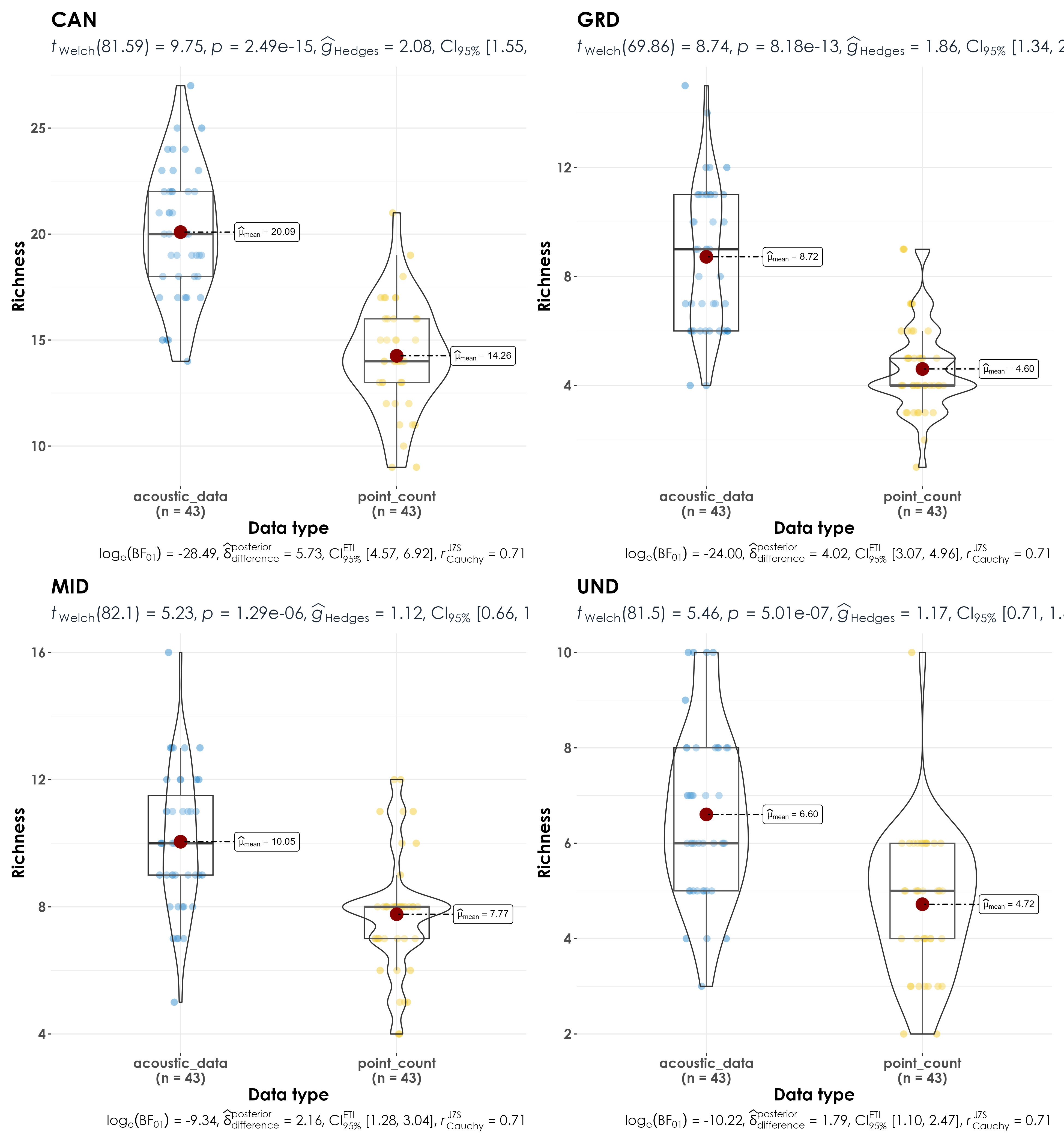
Significant differences in richness between acoustic data and point count data as a function of foraging guild
3.8 Stacked barplots for richness across foraging guilds
# reordering factors for plotting
foraging_richness$foraging_habit <- factor(foraging_richness$foraging_habit, levels = c("GRD","UND","MID","CAN"))

fig_stacked_forHabit <- ggbarstats(
  data = foraging_richness,
  x = foraging_habit,
  y = data_type,
  counts = richness,
  perc.k = 1,
  package = "ggsci",
  palette = "category10_d3",
  plotgrid.args = list(nrow = 3),
 ggplot.component = list(theme(text = element_text(family = "Century Gothic", size = 15, face = "bold"),plot.title = element_text(family = "Century Gothic",
      size = 18, face = "bold"),
      plot.subtitle = element_text(family = "Century Gothic",
      size = 15, face = "bold",color="#1b2838"),
      axis.title = element_text(family = "Century Gothic",
      size = 15, face = "bold"))))

ggsave(fig_stacked_forHabit, filename = "figs/fig_foragingHabit_stackedRichness.png", width = 13, height = 12, device = png(), units = "in", dpi = 300)
dev.off() 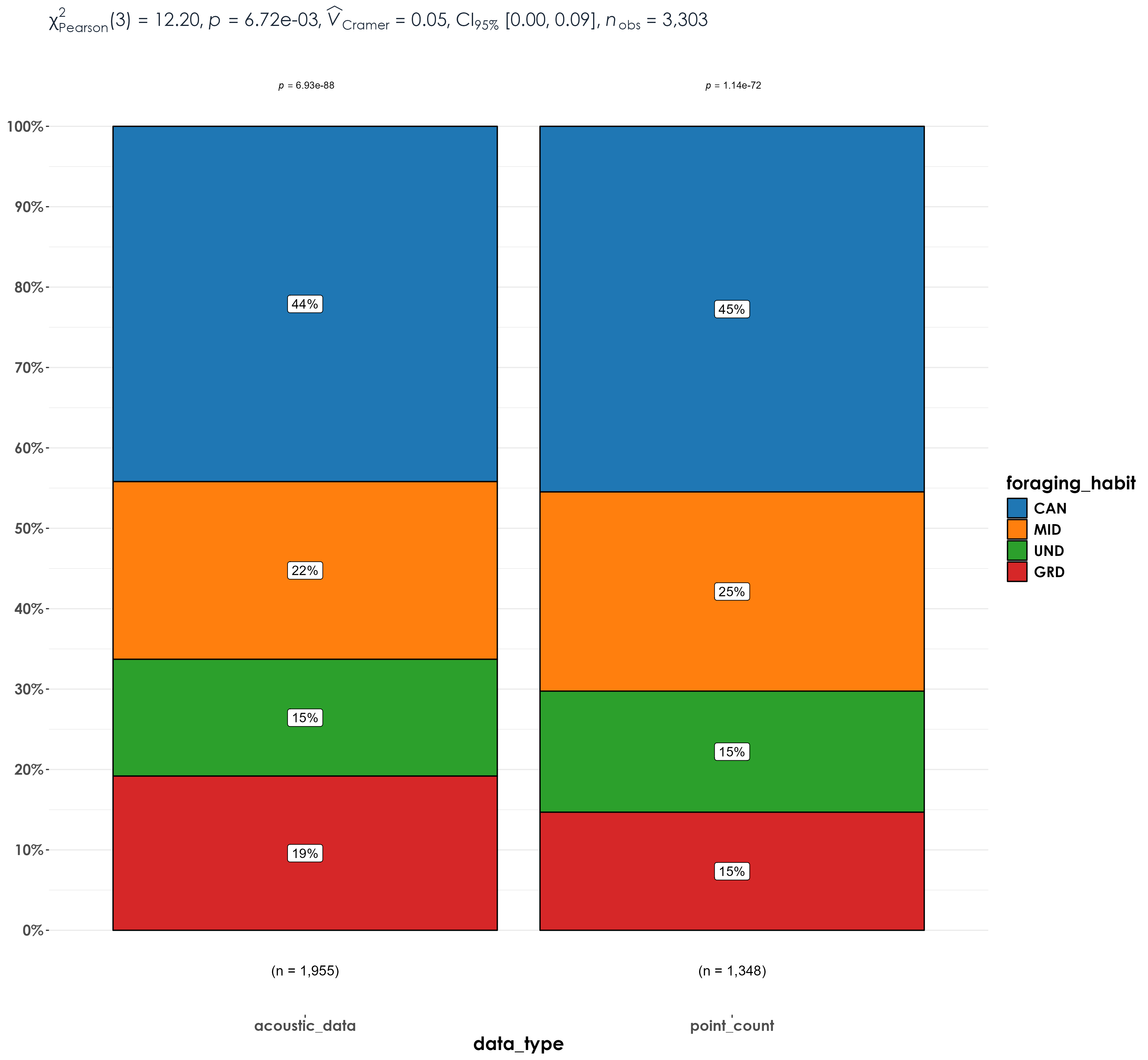
Stacked bar plots of richness by foraging guilds between point count data and acoustic data