Section 3 Vocal activity
In this script, we examine differences in vocal activity between dawn and dusk for each species.
3.3 Filtering acoustic data to ensure sampling periods are even across dawn and dusk
Since our recording schedule was uneven (6am to 10am in the morning and 4pm to 7pm in the evening), we filter acoustic data to retain recordings between 6am and 830am and recordings made between 4pm and 630pm so that the two sampling windows capture a similar amount of time right after dawn and right before dusk.
3.4 Vocal activity across time periods
A number of factors need to be considered in further analysis: accounting for time_of_day, observed_identity for example. However, we run analyses that account for differences in calling activity by species for dawn and dusk.
# sampling effort by time_of_day
effort <- acoustic_data %>%
  dplyr::select(site_id, date, time_of_day) %>%
  distinct() %>%
  arrange(time_of_day) %>%
  count(time_of_day) %>%
  rename(., nVisits = n)

# Above, we note that we had sampled ~145 site-date combinations at dawn, while ~230 site-date combinations were sampled at dusk

# total number of acoustic detections summarized across every 10-s audio file
# here, we estimate % detections at dawn and dusk, while accounting for sampling effort
vocal_act <- acoustic_data %>%
  group_by(time_of_day, eBird_codes) %>%
  summarise(detections = sum(number)) %>%
  left_join(., species_codes[, c(1, 2, 5)],
    by = "eBird_codes"
  ) %>%
  group_by(eBird_codes) %>%
  mutate(total_detections = sum(detections)) %>%
  mutate(percent_detections = (detections / total_detections) * 100) %>%
  ungroup()

## accouting for sampling effort and normalizing data
vocal_act <- vocal_act %>%
  left_join(., effort, by = "time_of_day") %>%
  mutate(normalized_detections = detections / nVisits) %>%
  group_by(eBird_codes) %>%
  mutate(total_normalized_detections = sum(normalized_detections)) %>%
  mutate(percent_normalized_detections = (normalized_detections / total_normalized_detections) * 100) %>%
  ungroup() %>%
  # in our case, we have 4 species which have 100% detections in dawn, Indian blackbird, Little spiderhunter, Oriental-Magpie Robin and Purple sunbird. For these, we add a additional row specifying no detections in dusk.

  add_row(
    time_of_day = "dusk", eBird_codes = "pursun4", detections = 0, scientific_name = "Cinnyris asiaticus", common_name = "Purple Sunbird", total_detections = 96, percent_detections = 0, normalized_detections = 0,
    percent_normalized_detections = 0, nVisits = 230, total_normalized_detections = 0.6620690
  ) %>%
  add_row(
    time_of_day = "dusk", eBird_codes = "eurbla2", detections = 0, scientific_name = "Turdus simillimus", common_name = "Indian Blackbird", total_detections = 179, percent_detections = 0, normalized_detections = 0,
    percent_normalized_detections = 0, nVisits = 230,
    total_normalized_detections = 1.2344828
  ) %>%
  add_row(
    time_of_day = "dusk", eBird_codes = "litspi1", detections = 0, scientific_name = "Arachnothera longirostra", common_name = "Little Spiderhunter", total_detections = 204, percent_detections = 0,
    normalized_detections = 0, nVisits = 230,
    percent_normalized_detections = 0,
    total_normalized_detections = 1.4068966
  ) %>%
  add_row(
    time_of_day = "dusk", eBird_codes = "magrob", detections = 0, scientific_name = "Copsychus saularis", common_name = "Oriental Magpie-Robin",
    total_detections = 119, percent_detections = 0,
    normalized_detections = 0, nVisits = 230,
    percent_normalized_detections = 0,
    total_normalized_detections = 0.6620690
  )

# for the sake of plotting, we will create a new variable
vocal_act$plot_percent <- ifelse(vocal_act$time_of_day == "dawn",
  -1 * vocal_act$percent_normalized_detections,
  vocal_act$percent_normalized_detections
)

# reordering legend appearance
vocal_act$time_of_day <- factor(vocal_act$time_of_day,
  levels = c("dawn", "dusk")
)

# figure of percent detections
fig_percent_detections <- ggplot(vocal_act, aes(
  x = reorder(common_name, -plot_percent),
  y = plot_percent,
  fill = time_of_day
)) +
  geom_text(aes(label = sprintf("%.1f", abs(plot_percent))),
    hjust = ifelse(vocal_act$plot_percent >= 0, 0, 1),
    size = 3
  ) +
  geom_bar(stat = "identity") +
  scale_fill_manual(values = c("#d95f02", "#1b9e77")) +
  scale_y_continuous(labels = function(x) sprintf("%.1f", abs(x)))  +
  coord_flip() +
  labs(
    y = "% Vocal Activity",
    x = "Species Common Name"
  ) +
  theme_bw() +
  theme(
    text = element_text(family = "Century Gothic", size = 14, face = "bold"), plot.title = element_text(
      family = "Century Gothic",
      size = 15, face = "bold"
    ),
    plot.subtitle = element_text(
      family = "Century Gothic",
      size = 15, face = "bold", color = "#1b2838"
    ),
    axis.title = element_text(
      family = "Century Gothic",
      size = 18, face = "bold"
    ),
    legend.position = "top",
    legend.title = element_blank(),
    legend.text = element_text(size = 10)
  )

ggsave(fig_percent_detections, filename = "figs/fig_percentDetections_species.png", width = 14, height = 16, device = png(), units = "in", dpi = 300)
dev.off()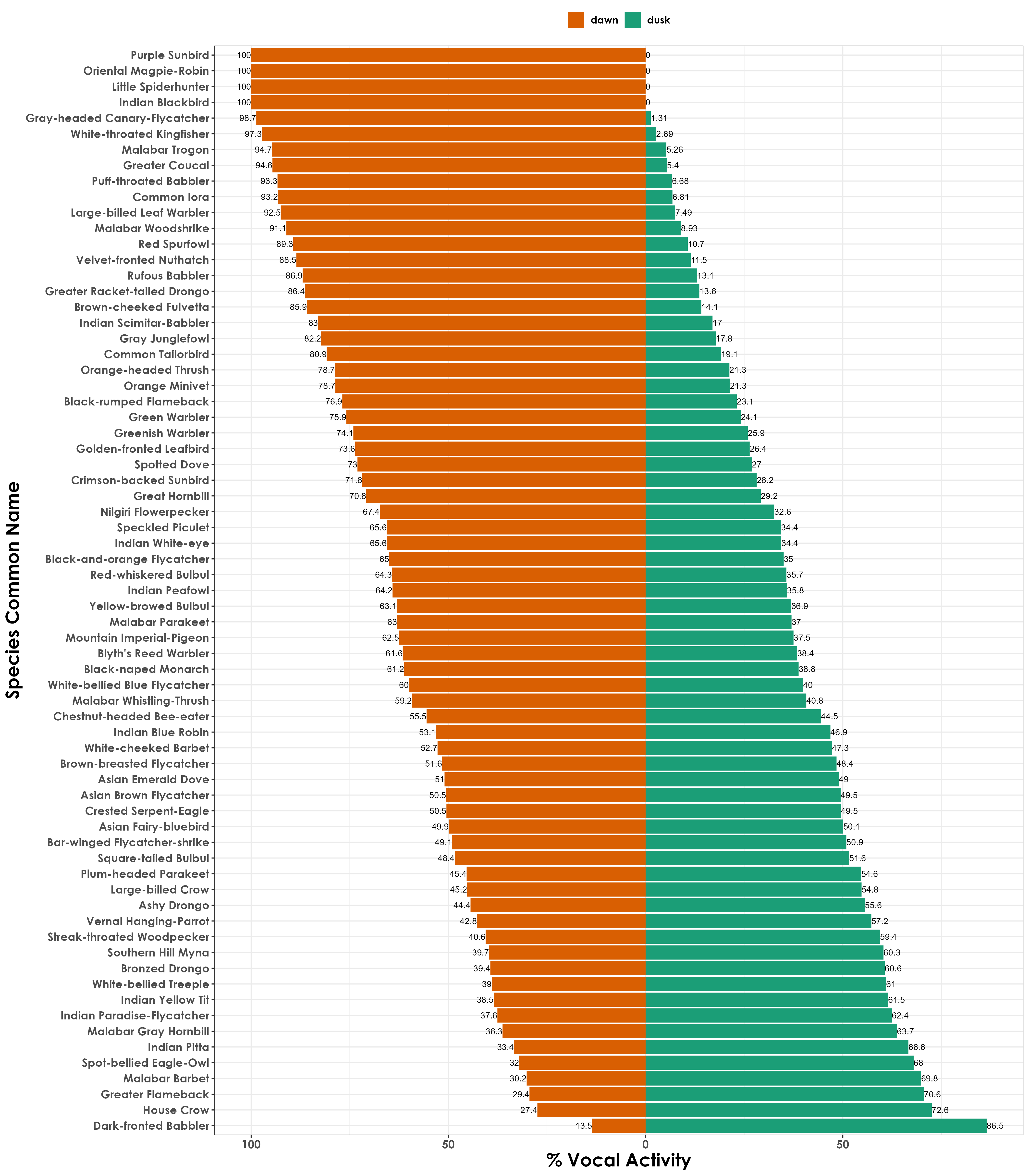
Species-specific differences in vocal activity across dawn and dusk
3.5 Is overall vocal activity much higher at dawn compared to dusk, across species?
fig_overall_vocal_act <- vocal_act %>%
  filter(time_of_day == "dawn") %>%
  ggbetweenstats(
    x = time_of_day,
    y = percent_normalized_detections,
    xlab = "Time of Day",
    ylab = "% Overall Vocal Activity at Dawn",
    pairwise.display = "significant",
    violin.args = list(width = 0),
    ggplot.component = list(theme(
      text = element_text(family = "Century Gothic", size = 14, face = "bold.italic"), plot.title = element_text(
        family = "Century Gothic",
        size = 15, face = "bold"
      ),
      plot.subtitle = element_text(
        family = "Century Gothic",
        size = 15, face = "bold", color = "#1b2838"
      ),
      axis.title = element_text(
        family = "Century Gothic",
        size = 18, face = "bold"
      )
    ))
  ) +
  coord_flip() +
  scale_y_reverse() +
  scale_color_manual(values = c("#d95f02", "#1b9e77"))

## Edits made to figure to show only data for dawn (since % activity is significantly higher than dusk

ggsave(fig_overall_vocal_act, filename = "figs/fig_percentDetections_overall.png", width = 14, height = 7, device = png(), units = "in", dpi = 300)
dev.off()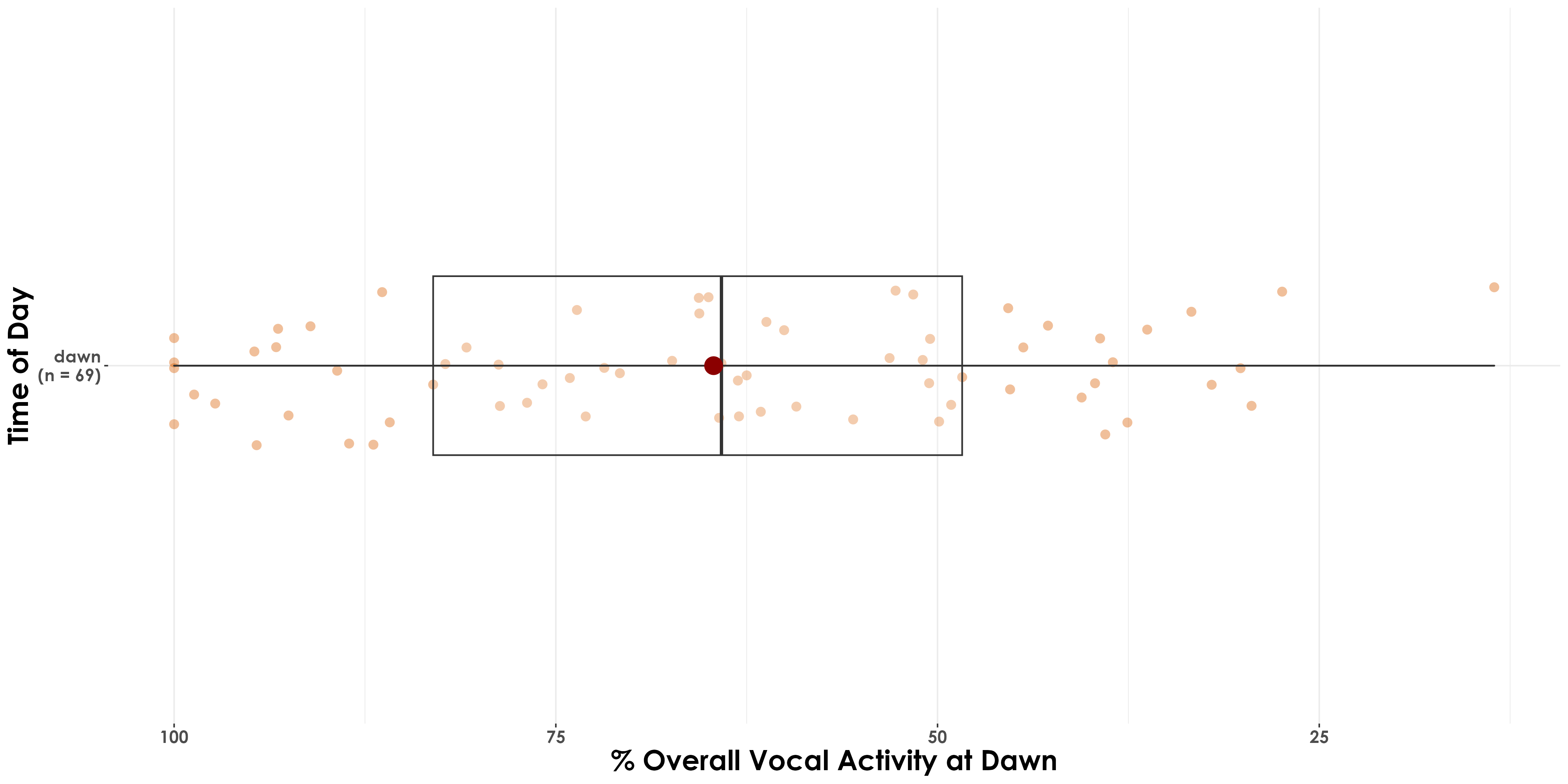
Overall, higher vocal activity was detected at dawn compared to dusk, across species.
3.6 Testing for differences in acoustic detections between dawn and dusk
Here, we see whether there are differences in the acoustic detections for each species between dawn and dusk.
stat.test <- vocal_act %>%
  pairwise_wilcox_test(percent_normalized_detections ~ time_of_day)

# We observe significant differences in vocal activity across species between dawn and dusk

# A tibble: 1 × 9
#  .y.        group1 group2    n1    n2 statistic        p    p.adj p.adj.signif
# <chr>      <chr>  <chr>  <int> <int>     <dbl>    <dbl>    <dbl> <chr>
# detections dawn   dusk      69    69     3192. 0.000549 0.000549 ***
3.7 Figure for publication
# Here, we will combine the above two figures created
library(patchwork)
fig_vocAct <- wrap_plots(fig_overall_vocal_act, fig_percent_detections,
  nrow = 2
) +
  plot_annotation(
    tag_levels = "a",
    tag_prefix = "(",
    tag_suffix = ")"
  ) +
  plot_layout(heights = c(1, 8))

ggsave(fig_vocAct, filename = "figs/fig01.png", width = 14, height = 20, device = png(), units = "in", dpi = 300)
dev.off()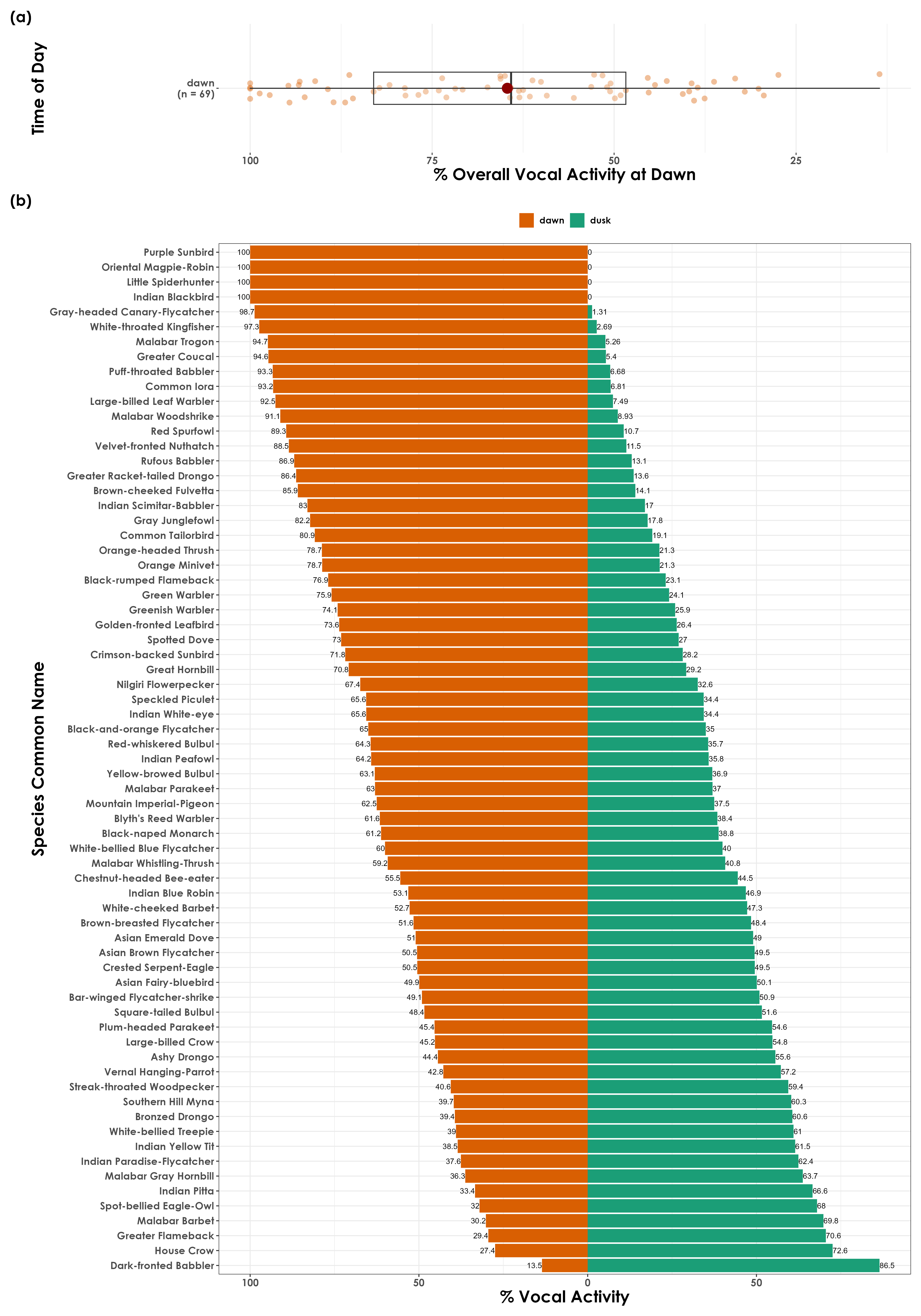
(a) Vocal activity was significantly higher at dawn compared to dusk across a tropical bird community in the Western Ghats. (b) Species-specific vocal activity across dawn and dusk.