Section 4 Frequency

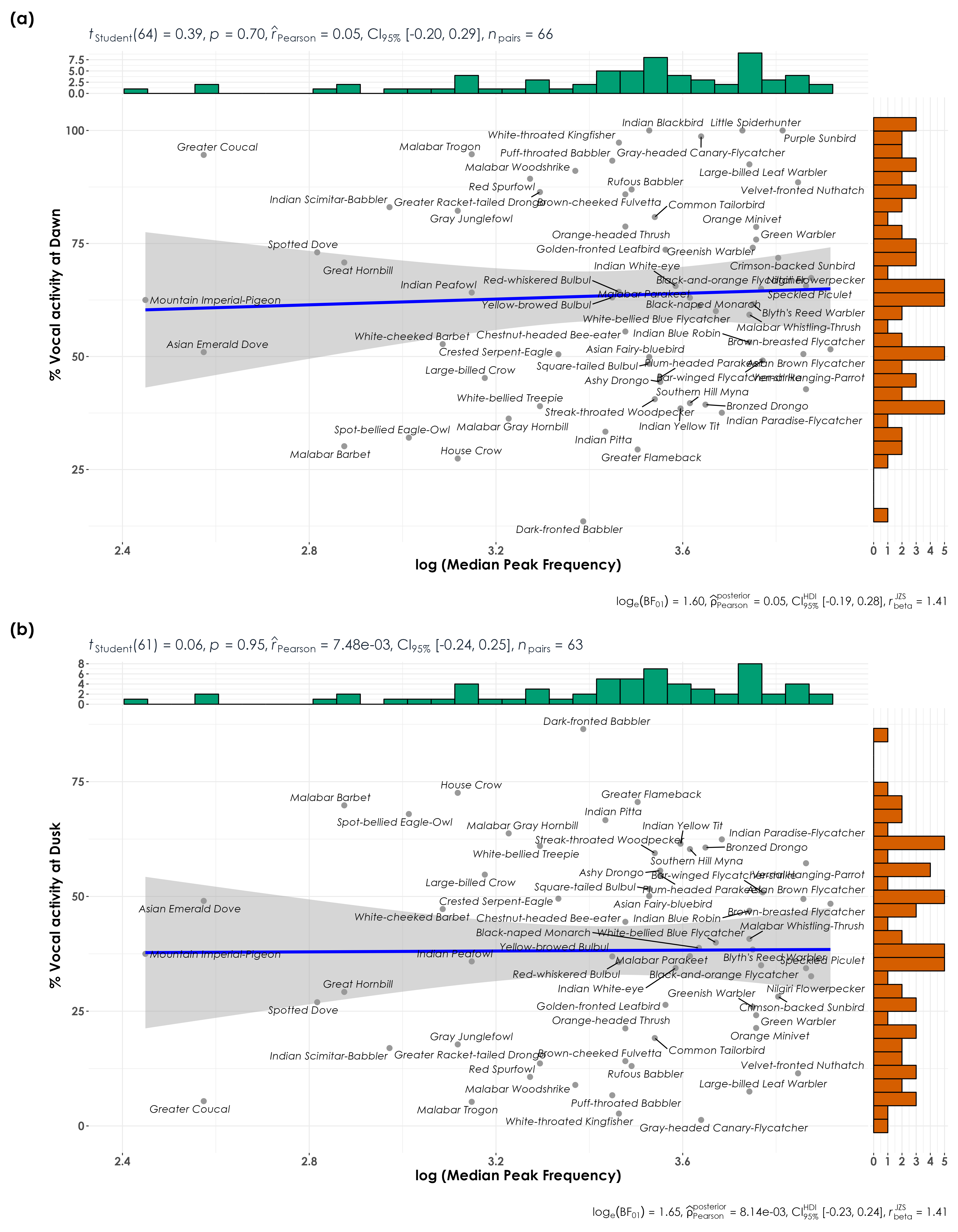
In this script, we examine differences in vocal activity between dawn and dusk for each species as a function of frequency. The expectation is that higher frequency vocalizers would call more at dawn compared to dusk, owing to better signal transmission in the morning.

4.1 Install necessary libraries

library(tidyverse)
library(dplyr)
library(stringr)
library(vegan)
library(ggplot2)
library(scico)
library(data.table)
library(extrafont)
library(ggstatsplot)
library(ggpubr)
library(ggrepel)

4.2 Load acoustic data and species scientific names data

acoustic_data <- read.csv("results/acoustic_data.csv")
species_codes <- read.csv("data/species-annotation-codes.csv")
freq <- read.csv("data/frequency-data.csv")

4.3 Filtering acoustic data to ensure sampling periods are even across dawn and dusk

Since our recording schedule was uneven (6am to 10am in the morning and 4pm to 7pm in the evening), we filter acoustic data to retain recordings between 6am and 830am and recordings made between 4pm and 630pm so that the two sampling windows capture a similar amount of time right after dawn and right before dusk.

dawn <- acoustic_data %>%
  group_by(time_of_day == "dawn") %>%
  filter(start_time >= 060000 & start_time <= 083000)

dusk <- acoustic_data %>%
  group_by(time_of_day == "dusk") %>%
  filter(start_time >= 160000 & start_time <= 183000)

acoustic_data <- bind_rows(dawn[, -10], dusk[, -10])

4.4 Vocal activity data

# sampling effort by time_of_day
effort <- acoustic_data %>%
  dplyr::select(site_id, date, time_of_day) %>%
  distinct() %>%
  arrange(time_of_day) %>%
  count(time_of_day) %>%
  rename(., nVisits = n)

# total number of acoustic detections summarized across every 10-s audio file
# here, we estimate % detections at dawn and dusk, while accounting for sampling effort
vocal_act <- acoustic_data %>%
  group_by(time_of_day, eBird_codes) %>%
  summarise(detections = sum(number)) %>%
  left_join(., species_codes[, c(1, 2, 5)],
    by = "eBird_codes"
  ) %>%
  group_by(eBird_codes) %>%
  mutate(total_detections = sum(detections)) %>%
  mutate(percent_detections = (detections / total_detections) * 100) %>%
  ungroup()

## accouting for sampling effort and normalizing data
vocal_act <- vocal_act %>%
  left_join(., effort, by = "time_of_day") %>%
  mutate(normalized_detections = detections / nVisits) %>%
  group_by(eBird_codes) %>%
  mutate(total_normalized_detections = sum(normalized_detections)) %>%
  mutate(percent_normalized_detections = (normalized_detections / total_normalized_detections) * 100) %>%
  ungroup()

4.5 Frequency data

We will extract the median peak frequency for each species. Note: For a total of 114 species, template recordings (varying from a minimum of 2 templates to 1910 templates per species) was extracted by Meghana P Srivathsa. While extracting median peak frequency, no distinction was made between songs and calls. We removed species that had very few templates (we only kept species that had a minimum of five frequency related measures).

# add standardized eBird codes to the frequency data
freq <- left_join(freq, species_codes[c(3, 5)],
  by = "species_annotation_codes"
)

# Only a total of 99 species are left after filtering species with very few templates
nTemplates_5 <- freq %>%
  group_by(eBird_codes) %>%
  count() %>%
  filter(n >= 5) %>%
  drop_na()

# left-join to remove species with less than five templates in the frequency dataset
freq_5 <- left_join(nTemplates_5[, 1], freq)

# calculate median peak frequency
median_pf <- freq_5 %>%
  group_by(eBird_codes) %>%
  summarise(median_peak_freq = median(peak_freq_in_Hz))

## join the frequency data to the vocal activity data
voc_freq <- left_join(vocal_act, median_pf, by = "eBird_codes") %>%
  drop_na()

## calculate the log of median peak frequency
voc_freq <- voc_freq %>%
  mutate(log_freq = log10(median_peak_freq))

# A total of 66 species were included and three species were excluded due to lack of data.

4.6 Visualization of % detections vs. median peak frequency

Here, we model the % of detections as a function of median peak frequency.

## creating two plots - one for dawn and one for dusk and using patchwork to combine them
fig_freq_dawn <- voc_freq %>%
  filter(time_of_day == "dawn") %>%
  ggscatterstats(
    data = .,
    x = log_freq,
    y = percent_normalized_detections,
    xlab = "log (Median Peak Frequency)\n",
    ylab = "\n % Vocal activity at Dawn",
    pairwise.display = "significant",
    package = "ggsci",
    palette = "default_jco",
    violin.args = list(width = 0),
    ggplot.component = list(theme(
      text = element_text(family = "Century Gothic", size = 15, face = "bold"), plot.title = element_text(
        family = "Century Gothic",
        size = 18, face = "bold"
      ),
      plot.subtitle = element_text(
        family = "Century Gothic",
        size = 15, face = "bold", color = "#1b2838"
      ),
      axis.title = element_text(
        family = "Century Gothic",
        size = 15, face = "bold"
      )
    ))
  ) +
  geom_text_repel(aes(label = common_name),
    family = "Century Gothic",
    fontface = "italic"
  )

fig_freq_dusk <- voc_freq %>%
  filter(time_of_day == "dusk") %>%
  ggscatterstats(
    data = .,
    x = log_freq,
    y = percent_normalized_detections,
    xlab = "log (Median Peak Frequency)\n",
    ylab = "\n % Vocal activity at Dusk",
    pairwise.display = "significant",
    package = "ggsci",
    palette = "default_jco",
    violin.args = list(width = 0),
    ggplot.component = list(theme(
      text = element_text(family = "Century Gothic", size = 15, face = "bold"), plot.title = element_text(
        family = "Century Gothic",
        size = 18, face = "bold"
      ),
      plot.subtitle = element_text(
        family = "Century Gothic",
        size = 15, face = "bold", color = "#1b2838"
      ),
      axis.title = element_text(
        family = "Century Gothic",
        size = 15, face = "bold"
      )
    ))
  ) +
  geom_text_repel(aes(label = common_name),
    family = "Century Gothic",
    fontface = "italic"
  )

library(patchwork)
fig_freq_vocAct <- wrap_plots(fig_freq_dawn, fig_freq_dusk,
  nrow = 2
) +
  plot_annotation(
    tag_levels = "a",
    tag_prefix = "(",
    tag_suffix = ")"
  )

ggsave(fig_freq_vocAct, filename = "figs/fig_peakFrequency_vs_detections.png", width = 14, height = 18, device = png(), units = "in", dpi = 300)
dev.off()

Pearson’s correlation test showed (a) no correlation between vocal activity at dawn and median peak frequency and (b) no correlation between vocal activity at dusk and median peak frequency. Both the effect sizes were not statistically significant.