Section 7 Territoriality

In this script, we examine the role of territoriality in vocal activity between dawn and dusk. The expectation is that highly territorial, weakly territorial and non-territorial species have higher vocal activity in dawn than dusk.

Highly territorial species are those which defend and maintain their territories throughout the year. Weakly territorial species are those which have broadly overlapping home ranges, or sometimes join mixed flocks without defined spatial ranges. Non-territorial species are those which do not defend territories, or defend very small areas around nest sites, or defend song or display posts only.

7.1 Loading necessary libraries

library(tidyverse)
library(dplyr)
library(stringr)
library(vegan)
library(ggplot2)
library(scico)
library(data.table)
library(extrafont)
library(ggstatsplot)
library(purrr)
library(ggpubr)
library(ggrepel)
library(ggdist)
library(gghalves)
library(rstatix)

7.2 Loading territoriality data

territoriality <- read.csv("data/territoriality-data.csv")

territoriality <- territoriality %>% dplyr::select(Species, Territory)
colnames(territoriality) <- c("scientific_name", "territory")

# Updating the scientific names of following species as per our dataset:
# Flame-throated bulbul- Rubigula gularis (earlier Pycnonotus gularis)
# Black eagle- Ictinaetus malaiensis (earlier Ictinaetus malayensis)
# Brown-capped pygmy woodpecker- Yungipicus nanus (earlier Dendrocopos nanus)
# Malabar barbet- Psilopogon malabaricus (earlier Megalaima malabarica)
# Dark-fronted babbler- Dumetia atriceps (earlier Rhopocichla atriceps)
# Greater flameback- Chrysocolaptes guttacristatus (earlier Chrysocolaptes lucidus)
# Indian blue robin- Larvivora brunnea (earlier Luscinia brunnea)
# Indian yellow tit- Machlolophus aplonotus (earlier Parus aplonotus)
# Jungle babbler- Argya striata (earlier Turdoides striata)
# Orange-headed thrush- Geokichla citrina (earlier Zoothera citrina)
# Rufous babbler- Argya subrufa (earlier Turdoides subrufa)
# Rufous woodpecker- Micropternus brachyurus (earlier Celeus brachyurus)
# Rusty-tailed flycatcher- Ficedula ruficauda (earlier Muscicapa ruficauda
# Spot-bellied eagle owl- Ketupa nipalensis (earlier Bubo nipalensis)
# Spotted dove- Spilopelia chinensis (earlier Stigmatopelia chinensis)
# Thick-billed warbler- Arundinax aedon (earlier Acrocephalus aedon)
# White-bellied flycatcher- Cyornis pallidipes (earlier Cyornis pallipes)
# White-cheeked barbet- Psilopogon viridis (earlier Megalaima viridis)
# Wayanad laughingthrush- Pterorhinus delesserti (earlier Garrulax delesserti)
# Yellow-browed bulbul- Iole indica (earlier Acritillas indica)

territoriality <- territoriality %>% mutate(scientific_name = recode(scientific_name, "Pycnonotus gularis" = "Rubigula gularis", "Ictinaetus malayensis" = "Ictinaetus malaiensis", "Dendrocopos nanus" = "Yungipicus nanus", "Megalaima malabarica" = "Psilopogon malabaricus", "Rhopocichla atriceps" = "Dumetia atriceps", "Chrysocolaptes lucidus" = "Chrysocolaptes guttacristatus", "Luscinia brunnea" = "Larvivora brunnea", "Parus aplonotus" = "Machlolophus aplonotus", "Turdoides striata" = "Argya striata", "Zoothera citrina" = "Geokichla citrina", "Turdoides subrufa" = "Argya subrufa", "Celeus brachyurus" = "Micropternus brachyurus", "Muscicapa ruficauda" = "Ficedula ruficauda", "Bubo nipalensis" = "Ketupa nipalensis", "Stigmatopelia chinensis" = "Spilopelia chinensis", "Acrocephalus aedon" = "Arundinax aedon", "Cyornis pallipes" = "Cyornis pallidipes", "Megalaima viridis" = "Psilopogon viridis", "Garrulax delesserti" = "Pterorhinus delesserti", "Acritillas indica" = "Iole indica"))

7.3 Load acoustic data and species scientific names data

acoustic_data <- read.csv("results/acoustic_data.csv")
species_codes <- read.csv("data/species-annotation-codes.csv")

7.4 Filtering acoustic data to ensure sampling periods are even across dawn and dusk

Since our recording schedule was uneven (6am to 10am in the morning and 4pm to 7pm in the evening), we filter acoustic data to retain recordings between 6am and 830am and recordings made between 4pm and 630pm so that the two sampling windows capture a similar amount of time right after dawn and right before dusk.

dawn <- acoustic_data %>%
  group_by(time_of_day == "dawn") %>%
  filter(start_time >= 060000 & start_time <= 083000)

dusk <- acoustic_data %>%
  group_by(time_of_day == "dusk") %>%
  filter(start_time >= 160000 & start_time <= 183000)

acoustic_data <- bind_rows(dawn[, -10], dusk[, -10])

7.5 Vocal activity across time periods

A number of factors need to be considered in further analysis: accounting for time_of_day, observed_identity for example. However, we run analyses that account for differences in calling activity by species for dawn and dusk.

# sampling effort by time_of_day
effort <- acoustic_data %>%
  dplyr::select(site_id, date, time_of_day) %>%
  distinct() %>%
  arrange(time_of_day) %>%
  count(time_of_day) %>%
  rename(., nVisits = n)

# Above, we note that we had sampled ~145 site-date combinations at dawn, while ~230 site-date combinations were sampled at dusk

# total number of acoustic detections summarized across every 10-s audio file
# here, we estimate % detections at dawn and dusk, while accounting for sampling effort
vocal_act <- acoustic_data %>%
  group_by(time_of_day, eBird_codes) %>%
  summarise(detections = sum(number)) %>%
  left_join(., species_codes[, c(1, 2, 5)],
    by = "eBird_codes"
  ) %>%
  group_by(eBird_codes) %>%
  mutate(total_detections = sum(detections)) %>%
  mutate(percent_detections = (detections / total_detections) * 100) %>%
  ungroup()

## accouting for sampling effort and normalizing data
vocal_act <- vocal_act %>%
  left_join(., effort, by = "time_of_day") %>%
  mutate(normalized_detections = detections / nVisits) %>%
  group_by(eBird_codes) %>%
  mutate(total_normalized_detections = sum(normalized_detections)) %>%
  mutate(percent_normalized_detections = (normalized_detections / total_normalized_detections) * 100) %>%
  ungroup() %>%
  # in our case, we have 4 species which have 100% detections in dawn, Indian blackbird, Little spiderhunter, Oriental-Magpie Robin and Purple sunbird. For these, we add a additional row specifying no detections in dusk.

  add_row(
    time_of_day = "dusk", eBird_codes = "pursun4", detections = 0, scientific_name = "Cinnyris asiaticus", common_name = "Purple Sunbird", total_detections = 96, percent_detections = 0, normalized_detections = 0,
    percent_normalized_detections = 0, nVisits = 230, total_normalized_detections = 0.6620690
  ) %>%
  add_row(
    time_of_day = "dusk", eBird_codes = "eurbla2", detections = 0, scientific_name = "Turdus simillimus", common_name = "Indian Blackbird", total_detections = 179, percent_detections = 0, normalized_detections = 0,
    percent_normalized_detections = 0, nVisits = 230,
    total_normalized_detections = 1.2344828
  ) %>%
  add_row(
    time_of_day = "dusk", eBird_codes = "litspi1", detections = 0, scientific_name = "Arachnothera longirostra", common_name = "Little Spiderhunter", total_detections = 204, percent_detections = 0,
    normalized_detections = 0, nVisits = 230,
    percent_normalized_detections = 0,
    total_normalized_detections = 1.4068966
  ) %>%
  add_row(
    time_of_day = "dusk", eBird_codes = "magrob", detections = 0, scientific_name = "Copsychus saularis", common_name = "Oriental Magpie-Robin",
    total_detections = 119, percent_detections = 0,
    normalized_detections = 0, nVisits = 230,
    percent_normalized_detections = 0,
    total_normalized_detections = 0.6620690
  )

7.6 Join the vocal_activity data and territoriality data

vocal_act <- vocal_act %>%
  left_join(territoriality, by = "scientific_name") %>%
  dplyr::mutate(territory_cat = case_when(territory %in% "3" ~ "Highly territorial", territory %in% "2" ~ "Weakly territorial", territory %in% "1" ~ "Non-territorial"))

There are 19 highly territorial, 11 non-territorial and 39 weakly territorial species in both dawn and dusk.

7.7 Testing the differences between territoriality categories using Wilcoxon test

Here, we see whether there are differences in the vocal activity among highly territorial, weakly territorial and non-territorial species in dawn and dusk individually.

stat.test <- vocal_act %>%
  group_by(time_of_day) %>%
  wilcox_test(percent_normalized_detections ~ territory_cat)

Vocal activity is not significantly different across categories of territoriality.
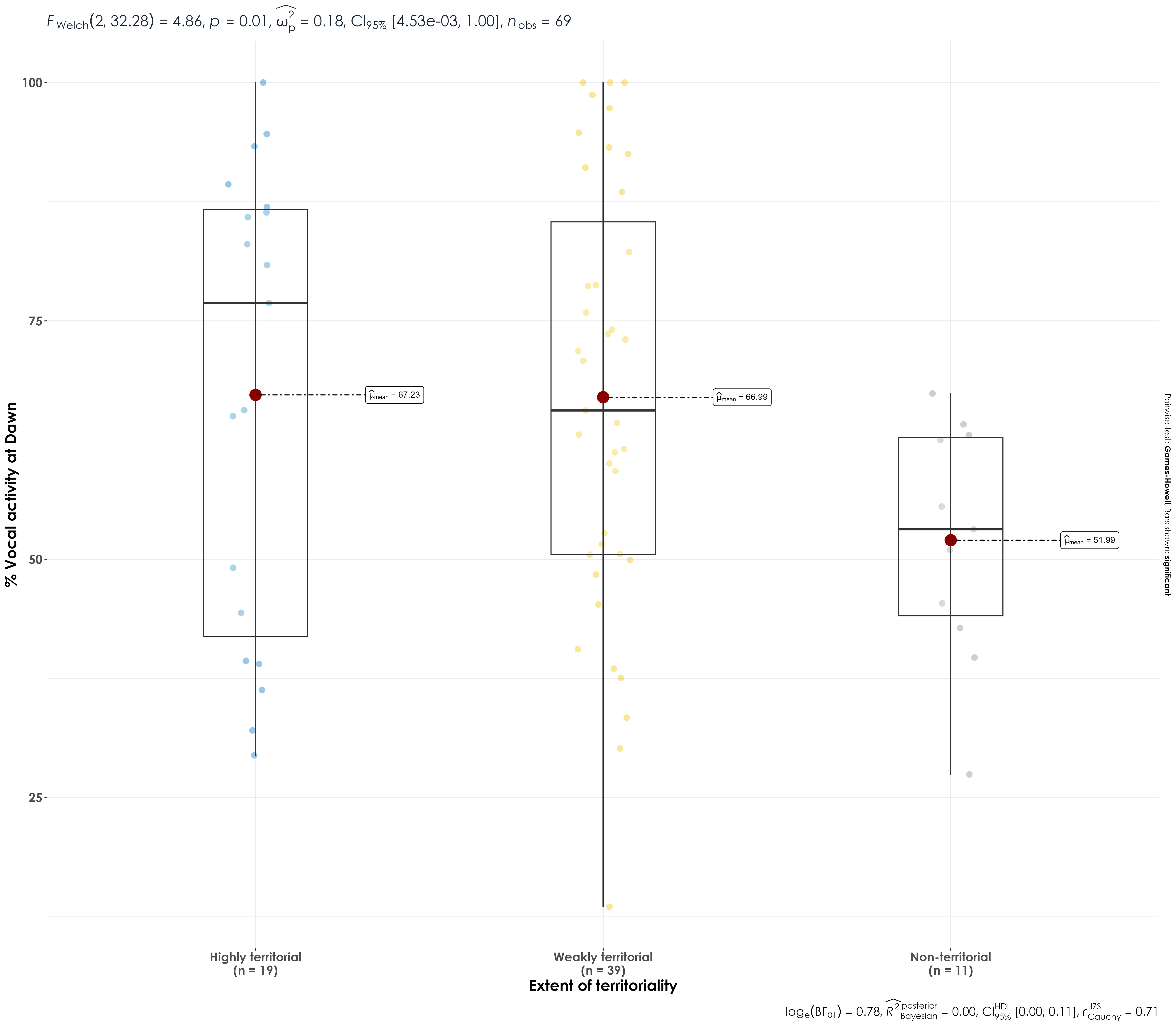
## Comparing dawn vocal activity between categories of territoriality

## between dawn and dusk
fig_terr_vocAct <- vocal_act %>%
  filter(time_of_day == "dawn") %>%
  mutate(territory_cat = fct_relevel(
    territory_cat,
    "Highly territorial", "Weakly territorial", "Non-territorial"
  )) %>%
  ggbetweenstats(
    x = territory_cat,
    y = percent_normalized_detections,
    xlab = "Extent of territoriality",
    ylab = "% Vocal activity at Dawn",
    pairwise.display = "significant",
    package = "ggsci",
    palette = "default_jco",
    violin.args = list(width = 0),
    ggplot.component = list(theme(
      text = element_text(family = "Century Gothic", size = 15, face = "bold"), plot.title = element_text(
        family = "Century Gothic",
        size = 18, face = "bold"
      ),
      plot.subtitle = element_text(
        family = "Century Gothic",
        size = 15, face = "bold", color = "#1b2838"
      ),
      axis.title = element_text(
        family = "Century Gothic",
        size = 15, face = "bold"
      )
    ))
  )

ggsave(fig_terr_vocAct, filename = "figs/fig_percentDetections_vs_territoriality.png", width = 16, height = 14, device = png(), units = "in", dpi = 300)
dev.off()

Weakly territorial species were significantly more dawn shifted than non-territorial species at dawn.