Section 11 Non-metric multidimensional scaling of bird species detections
Here, we are interested not only in comparing univariate descriptors of communities, like diversity, but also in how the constituent species — or the composition — changes from one community to the next.
One tool to do this is non-metric multidimensional scaling, or NMDS. The goal of NMDS is to collapse information from multiple dimensions (e.g, from multiple communities, sites, etc.) into just a few, so that they can be visualized and interpreted. Unlike other ordination techniques that rely on (primarily Euclidean) distances, such as Principal Component Analysis, NMDS uses rank orders, and thus is an extremely flexible technique that can accommodate a variety of different kinds of data (The text above was copied from the link below).
NMDS does not use the absolute abundances of species in communities, but rather their rank orders. The use of ranks omits some of the issues associated with using absolute distance (e.g., sensitivity to transformation), and as a result is much more flexible technique that accepts a variety of types of data. (It’s also where the “non-metric” part of the name comes from).
A wonderful tutorial is presented in this link: https://jonlefcheck.net/2012/10/24/nmds-tutorial-in-r/
11.1 Install required libraries
library(tidyverse)
library(dplyr)
library(stringr)
library(vegan)
library(ggplot2)
library(scico)
library(psych)
library(ecodist)
library(RColorBrewer)
library(ggforce)
library(ggalt)
library(patchwork)
library(sjPlot)

# Source any custom/other internal functions necessary for analysis
source("code/01_internal-functions.R")
11.2 Load the necessary data for NMDS calculations
# We load the subset data
datSubset <- read.csv("results/datSubset.csv")

# Load species-trait data to essentially check for associations by habitat type
trait_dat <- read.csv("data/species-trait-dat.csv")

# Site-summary (Number of detections across all sites)
datSummary <- datSubset %>%
  group_by(Site, Restoration.type) %>%
  transform() %>% replace(is.na(.), 0) %>%
  summarise_at(.vars = vars(c("IP":"HSWP")),.funs = sum)

# richness across sites (converting detections to 1)
richness <- datSummary %>%
  mutate_at(vars(c("IP":"HSWP")),~ replace(., . > 0, 1)) %>%
  rowwise() %>%
  mutate(richness = sum(c_across(IP:HSWP))) %>%
  dplyr::select(Site, Restoration.type, richness)
11.3 Preparing dataframe of traits and species to be used for NMDS later on
# Calculate the overall number of detections for each site. Here, we include dates, since each visit can explain the extrapolation of species richness when jackknife estimates are extracted.

nDetections_site_date <- datSubset %>%
  group_by(Site, Restoration.type, Date) %>%
  transform() %>% replace(is.na(.), 0) %>%
  summarise_at(.vars = vars(c("IP":"HSWP")),.funs = sum)

# Combine the nDetections and trait based data to obtain a dataframe for further analysis

nDetections_trait <- nDetections_site_date %>%
  pivot_longer(cols=IP:HSWP, names_to="Species_Code", values_to="count") %>%
  left_join(.,trait_dat, by=c("Species_Code"="species_annotation_codes")) %>%
  mutate(forRichness = case_when(count>0 ~ 1,count==0 ~ 0)) %>%
  rename(., nDetections = count)
11.4 Preparing a dataframe of detections to run ordinations
# We will prepare a community matrix data that can be used to run dissimilarity indices

nmdsDat <- nDetections_trait %>%
  dplyr::select(Site, Species_Code, nDetections, Restoration.type) %>%
  group_by(Species_Code, Site, Restoration.type) %>%
  summarise (totDetections = sum(nDetections)) %>%
  arrange(Restoration.type) %>%
  pivot_wider (names_from = Species_Code, values_from = totDetections, values_fill = list(totDetections=0))

# Convert to matrix form
nmdsDatMatrix <- as.matrix(nmdsDat[, 3:ncol(nmdsDat)])
11.5 Bray-Curtis dissimilarity index
Run a bray-curtis dissimilarity index and identify least stressed configuration for the ordinations. Bray-curtis is a statistic used to quantify the compositional dissimilarity between two different sites, based on counts at each site. Ecologists use the Bray-Curtis dissimilarity calculation, which has a number of ideal properties: 1. It is invariant to changes in units. 2. It is unaffected by additions/removals of species that are not present in two communities. 3. It is unaffected by the addition of a new community. 4. It can recognize differences in total abundances when relative abundances are the same.
Please note that this link provides more information on NMDS: http://strata.uga.edu/8370/lecturenotes/multidimensionalScaling.html
# Run a bray-curtis dissimilarity index and use metaMDS function from vegan to run ordinations

disBrayCurtis <- vegdist(nmdsDatMatrix, method = "bray")

nmdsBrayCurtis <- vegdist (nmdsDatMatrix, method = "bray") %>%
  metaMDS (nmdsBrayCurtis, k=6)

# extract nmds scores
nmdsScores <- as.tibble(scores(nmdsBrayCurtis, display = "site"))

# Write the scores to a separate .csv
write.csv(nmdsScores, "data/nmdsBrayCurtis-bird-detections.csv", row.names = F)

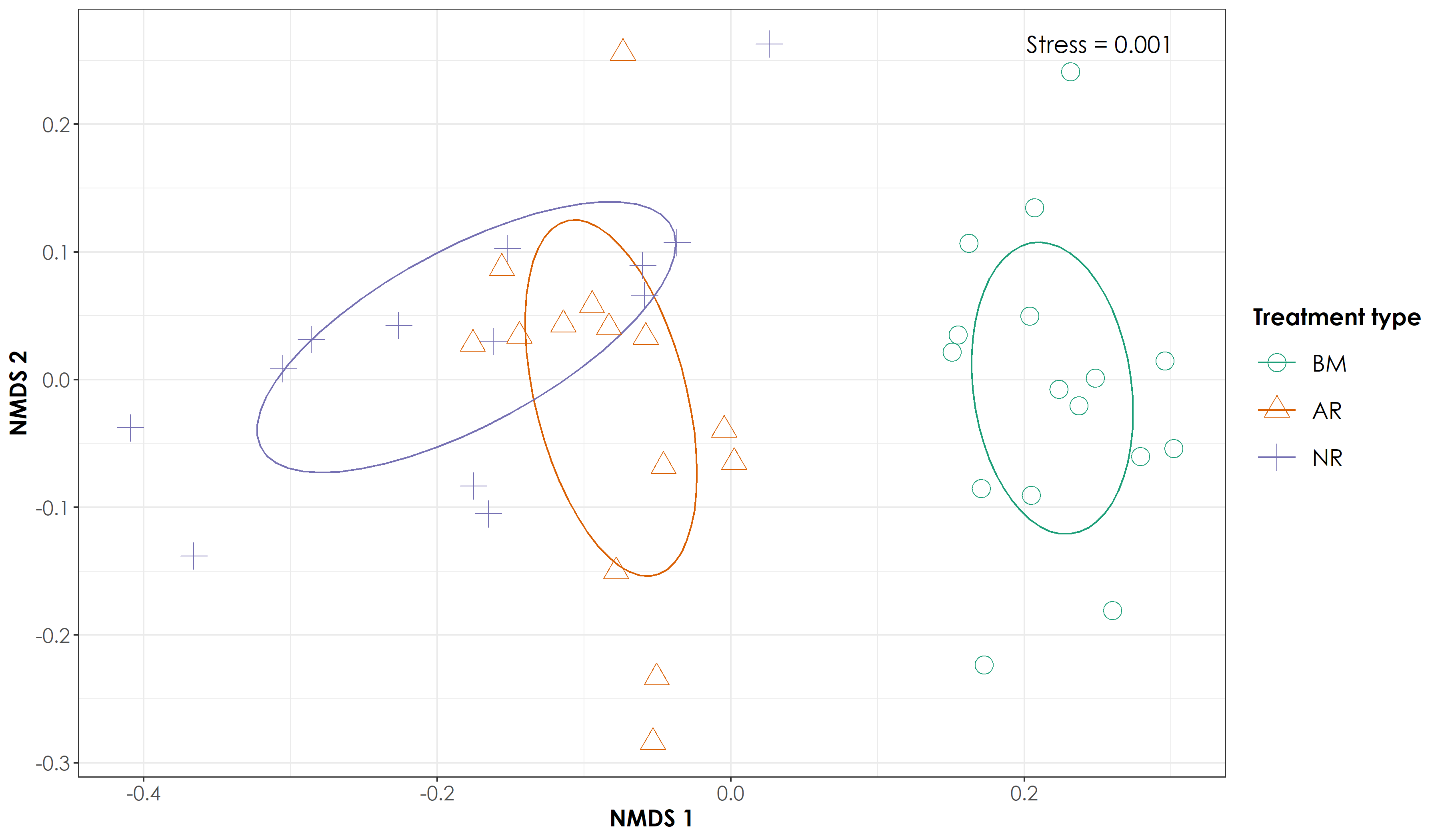
# With the above analysis, we note the stress is 0.001537865. However, if stress is high, we should reposition the points in 2 dimensions in the direction of decreasing stress, and repeat until stress is below some threshold.**A good rule of thumb: stress < 0.05 provides an excellent representation in reduced dimensions, < 0.1 is great, < 0.2 is good/ok, and stress < 0.3 provides a poor representation.** To reiterate: high stress is bad, low stress is good!
11.6 Plotting the NMDS scores
# First let's add the treatment type back to the nmds scores
nmdsScores$Restoration.type <- nmdsDat$Restoration.type

# Add a custom set of colors
mycolors <- c(brewer.pal(name="Dark2", n = 3), brewer.pal(name="Paired", n = 3))

# reordering factors for plotting
nmdsScores$Restoration.type <- factor(nmdsScores$Restoration.type, levels = c("Benchmark", "Active", "Passive"))

fig_nmds <- ggplot(data=nmdsScores) +
  stat_ellipse(aes(x=NMDS1,y=NMDS2,colour=Restoration.type),level = 0.50) +
  geom_point(aes(x=NMDS1,y=NMDS2,shape=Restoration.type,colour=Restoration.type),size=5) +
  theme_bw() +
  scale_x_continuous(name="NMDS 1") +
  scale_y_continuous(name="NMDS 2") +
  scale_shape_manual("Treatment type",values= 1:length(unique(nmdsScores$Restoration.type)), labels=c("BM","AR","NR"))+
  scale_color_manual("Treatment type",values=mycolors, labels=c("BM","AR","NR"))+
  theme(axis.title = element_text(family="Century Gothic",
                                    size = 14, face = "bold"),
        axis.text = element_text(family="Century Gothic",
                                    size = 12),
        legend.title = element_text(family="Century Gothic",
                                    size = 14, face = "bold"),
        legend.key.size = unit(1,"cm"),
        legend.text = element_text(family="Century Gothic",size = 14)) +
   annotate(geom = "text", x = max(nmdsScores$NMDS1), y = max(nmdsScores$NMDS2),  label = "Stress = 0.001", hjust = 1, family = "Century Gothic", size=5)

ggsave(fig_nmds, filename = "figs/fig_nmds_birdDetections.png", width=12, height=7,device = png(), units="in", dpi = 300); dev.off()
AR sites are transitioning toward BM sites
11.7 Main text Figure 5
# reload previous figures to create part A and B for the main text Fig. 4

library(patchwork)

fig_prop_ordinations <-
  wrap_plots(fig_propRF, fig_propOC, fig_nmds,
    design = 'AB
              CC'
  ) +
  plot_annotation(
    tag_levels = "a",
    tag_prefix = "(",
    tag_suffix = ")"
  )

# Expand the width to avoid compression
ggsave(fig_prop_ordinations, filename = "figs/fig05.png", width=15, height=12,device = png(), units="in", dpi = 300); dev.off()
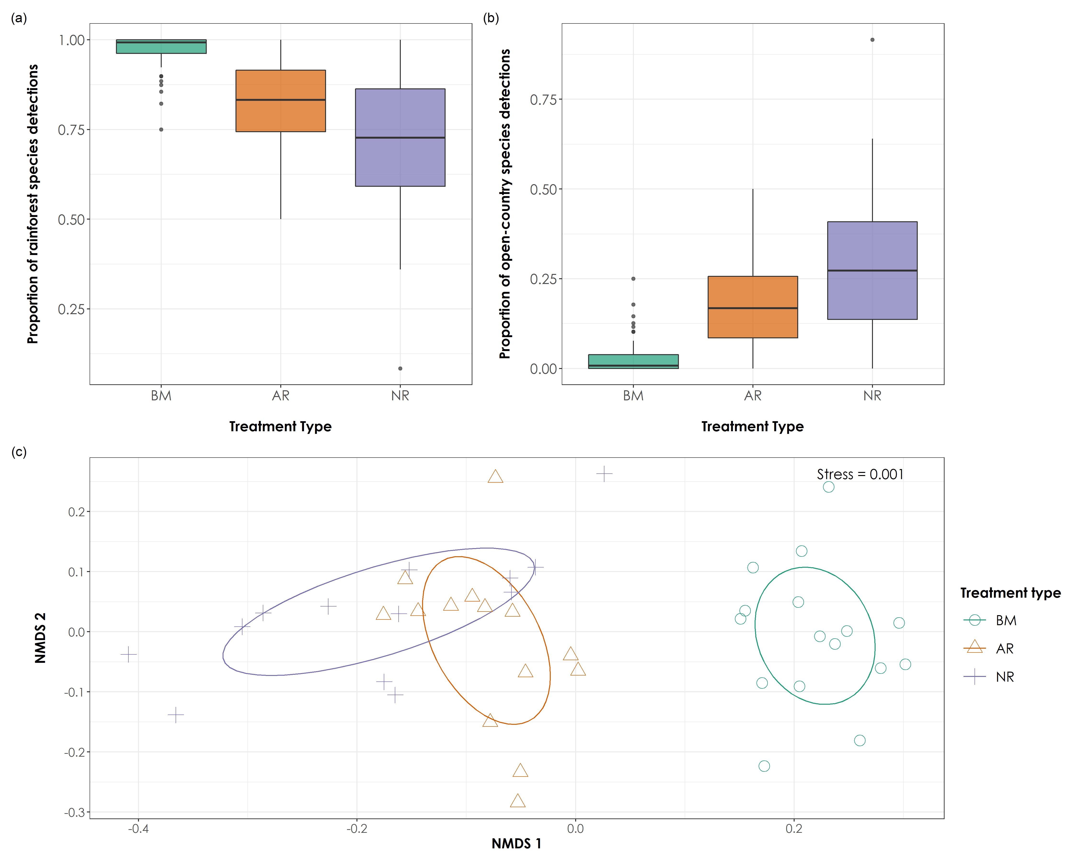
Proportion of acoustic detections of rainforest and open-country bird species and NMDS ordination results of bird species detections (a) We observed significant differences in the proportion of rainforest bird species detections across each of the three treatment types (Tukey HSD test, P < 0.05). BM sites had the highest proportion of rainforest bird species detections (mean ± SD: 0.97 ± 0.04), followed by AR sites (mean ± SD: 0.81 ± 0.12), and NR sites (mean ± SD: 0.71 ± 0.17). (b) We observed significant differences in the proportion of open-country bird species detections across each of the three treatment type (Tukey HSD test, P < 0.05). NR sites had the highest proportion of open-country bird species detections (mean ± SD: 0.28 ± 0.17), followed by AR sites (mean ± SD: 0.18 ± 0.12), and BM sites (mean ± SD: 0.02 ± 0.04). (b) The ordination analysis of bird detections data (stress = 0.001) revealed distinct clusters of BM sites, but relatively loose clusters for AR and NR sites. However, AR sites occupied an intermediate position between BM and NR sites, indicating a direction of change in bird community composition toward BM sites. In the above figure, BM = undisturbed benchmark rainforest sites, AR = Actively restored forest sites and NR = Naturally regenerating forest sites.
11.8 Testing multivariate homogeneity of group dispersions
One measure of multivariate dispersion (variance) for a group of samples is to calculate the average distance of group members to the group centroid or spatial median in multivariate space. To test if the dispersions (variances) of one or more groups are different, the distances of group members to the group centroid are subject to ANOVA.
Betadisper tests whether two or more groups (for example, restored and unrestored sites) are homogeneously dispersed in relation to their species in studied samples. This test can be done to see if one group has more compositional variance than another. Moreover, homogeneity of dispersion among groups is very advisable to have if you want to test if two or more groups have different compositions, which is tested by adonis.
nmdsVariance <- betadisper(disBrayCurtis, group = nmdsDat$Restoration.type)
nmdsVariance

anova(nmdsVariance)
permutest(nmdsVariance, pairwise = TRUE, permutations = 999)
TukeyHSD(nmdsVariance)

# These results suggest that there is no difference in within-group variance between one group and another
11.9 Visualizing the multivariate homogeneity of group dispersions
The below lines of code have been adapted from: https://chrischizinski.github.io/rstats/adonis/
# extract the centroids and the site points in multivariate space.
centroids <-data.frame(grps=rownames(nmdsVariance$centroids),
                       data.frame(nmdsVariance$centroids))
vectors <- data.frame(group=nmdsVariance$group,
                      data.frame(nmdsVariance$vectors))

# to create the lines from the centroids to each point we will put it in a format that ggplot can handle
seg.data<-cbind(vectors[,1:3],centroids[rep(1:nrow(centroids),as.data.frame(table(vectors$group))$Freq),2:3])
names(seg.data)<-c("group","v.PCoA1","v.PCoA2","PCoA1","PCoA2")

# create the convex hulls of the outermost points
grp1.hull <- seg.data[seg.data$group=="Active",1:3][chull(seg.data[seg.data$group=="Active",2:3]),]
grp2.hull <- seg.data[seg.data$group=="Benchmark",1:3][chull(seg.data[seg.data$group=="Benchmark",2:3]),]
grp3.hull <- seg.data[seg.data$group=="Passive",1:3][chull(seg.data[seg.data$group=="Passive",2:3]),]
all.hull <- rbind(grp1.hull,grp2.hull,grp3.hull)

# plot the panel and convex hulls
fig_hull <- ggplot() +
  geom_polygon(data= all.hull,aes(x=v.PCoA1,y=v.PCoA2),colour="black",alpha=0,linetype="dashed") +
  geom_segment(data=seg.data,aes(x=v.PCoA1,xend=PCoA1,y=v.PCoA2,yend=PCoA2),alpha=0.30) +
  geom_point(data=centroids[,1:3], aes(x=PCoA1,y=PCoA2,shape=grps),size=4,colour="red") +
  geom_point(data=seg.data, aes(x=v.PCoA1,y=v.PCoA2,shape=group),size=2) +
  labs(title="All",x="",y="") +
  #coord_cartesian(xlim = c(-0.2,0.2), ylim = c(-0.25,0.2)) +
  theme_bw() +
  theme(legend.position="none")
11.10 Testing compositional dissimilarity between groups
We will do this by using the vegan::adonis() function which allows you to run permutational multivariate analysis of variance using distance matrices. In the above figure, the NMDS confidence ellipses suggest that there is a significant difference between benchmark and passive-active sites, but no difference between active and passive sites. Adonis works by first finding the centroids for each group and then calculates the squared deviations of each of site to that centroid. Then significance tests are performed using F-tests based on sequential sums of squares from permutations of the raw data. Please note that adonis analyzes and partitions sums of squares using distance matrices. It can be thought of as an ANOVA using distance matrices (analogous to MANOVA - multivariate analysis of variance). Therefore, it is used to test if two or more groups have similar compositions.
# We will use the NMDS scores for axis 1 and axis 2 to test for compositional dissimilarity
groups <- nmdsScores$Restoration.type

adonisNMDS <- adonis2(nmdsDatMatrix ~ groups, method="bray",perm=999)
adonisNMDS

# The results suggest that there are significant compositional differences between groups.
11.11 Separate analysis: Instead of using bird detections, using richness to run nmds ordinations
nmdsDatRichness <- datSummary %>%
  mutate_at(vars(c("IP":"HSWP")),~ replace(., . > 0, 1))

# Convert to matrix form
nmdsDatMatrixRichness <- as.matrix(nmdsDatRichness[, 3:ncol(nmdsDatRichness)])

# Run a bray-curtis dissimilarity index and use metaMDS function from vegan to run ordinations

disBrayCurtisRichness <- vegdist(nmdsDatMatrixRichness, method = "bray")

nmdsBrayCurtisRichness <- vegdist(nmdsDatMatrixRichness, method = "bray") %>%   metaMDS (nmdsBrayCurtisRichness, k=6)

# extract nmds scores
nmdsScoresRichness <- as.tibble(scores(nmdsBrayCurtisRichness))

# plot the data
# First let's add the treatment type back to the nmds scores
nmdsScoresRichness$Restoration.type <- nmdsDatRichness$Restoration.type

# Add a custom set of colors
mycolors <- c(brewer.pal(name="Dark2", n = 3), brewer.pal(name="Paired", n = 3))

# reordering factors for plotting
nmdsScoresRichness$Restoration.type <- factor(nmdsScoresRichness$Restoration.type, levels = c("Benchmark", "Active", "Passive"))

fig_nmds_richness <- ggplot(data=nmdsScoresRichness) +
  stat_ellipse(aes(x=NMDS1,y=NMDS2,colour=Restoration.type),level = 0.50) +
  geom_point(aes(x=NMDS1,y=NMDS2,shape=Restoration.type,colour=Restoration.type),size=4) +
  theme_bw() +
  scale_x_continuous(name="NMDS 1") +
  scale_y_continuous(name="NMDS 2") +
  scale_shape_manual("Treatment type",values= 1:length(unique(nmdsScoresRichness$Restoration.type)), labels=c("BM","AR","NR"))+
  scale_color_manual("Treatment type",values=mycolors, labels=c("BM","AR","NR"))+
  theme(axis.title = element_text(family="Century Gothic",
                                    size = 14, face = "bold"),
        axis.text = element_text(family="Century Gothic",
                                    size = 12),
        legend.title = element_text(family="Century Gothic",
                                    size = 14, face = "bold"),
        legend.key.size = unit(1,"cm"),
        legend.text = element_text(family="Century Gothic",size = 14)) +
   annotate(geom = "text", x = max(nmdsScoresRichness$NMDS1), y = max(nmdsScoresRichness$NMDS2),  label = "Stress = 0.1", hjust = 1, family = "Century Gothic", size=5)

ggsave(fig_nmds_richness, filename = "figs/fig_nmds_birdRichness.png", width=12, height=7,device = png(), units="in", dpi = 300); dev.off()
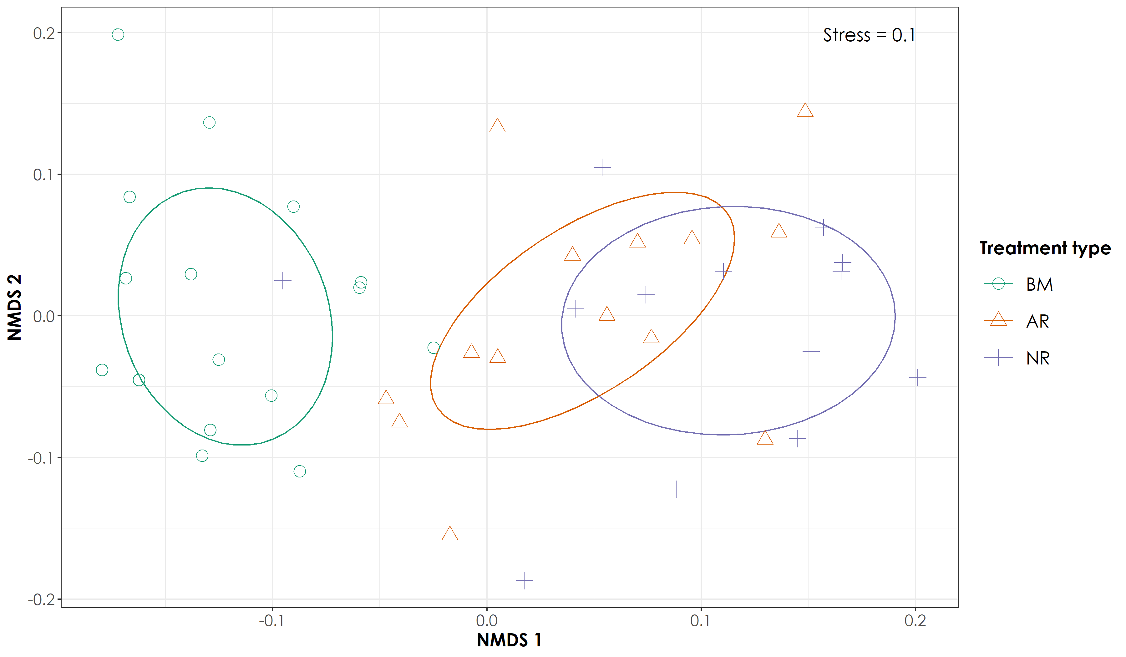
Similar results as that of bird species detections were observed.