Section 6 Generalized linear mixed modeling (acoustic space use and vegetation data)
In this script, we run generalized linear models to test the association between acoustic space use values and restoration type. In addition, we run generalized linear mixed models to test associations between acoustic space use and habitat (vegetation structure) using site-pair name (actively restored and naturally regenerating were specified to be paired) and repeat visits as random effects.
6.1 Install required libraries
library(tidyverse)
library(dplyr)
library(stringr)
library(vegan)
library(ggplot2)
library(scico)
library(psych)
library(rcompanion)
library(multcomp)
library(lme4)
library(ggpubr)
library(sjPlot)
library(RColorBrewer)
library(extrafont)

# Source any custom/other internal functions necessary for analysis
source("code/01_internal-functions.R")
6.2 Load necessary data for statistical modeling
# load list of sites
sites <- read.csv("data/list-of-sites.csv") %>%
  dplyr::select("Site.code","Restoration.type") %>%
  filter(Site.code != "OLCAP5B")

# load the entire asu data across all sites and days computed
sitebyDayAsu <- read.csv("results/site-by-day-asu.csv")

# separate by Site and Date
sitebyDayAsu <- separate(sitebyDayAsu, col = Site_Day, into = c("Site", "Date"), sep = "_")

# Add restoration type column to the space use data
sitebyDayAsu <- left_join(sitebyDayAsu, sites, by=c("Site"="Site.code"))

# scale values per site/date for comparison between sites and treatment types
sitebyDayAsu <- sitebyDayAsu %>%
  group_by(Site, Date, Restoration.type) %>%
  mutate(f.cont.scaled = range01(f.cont))

# computing total number of days for which space use has been computed for each site (some sites have very few days. Eg. OLV110R, else rest have 5 days of audio data each)
nSites_Days <- sitebyDayAsu %>%
  dplyr::select(Site, Date, Restoration.type) %>%
  distinct() %>%
  group_by(Site) %>%
  count()

# Let's look at data by restoration type
# This suggests that we have more data for benchmark sites relative to the other two treatment types
nDays_siteType <- sitebyDayAsu %>%
  dplyr::select(Site, Date, Restoration.type) %>%
  distinct() %>%
  group_by(Restoration.type) %>%
  count()

# Separate analysis: space use during diurnal and nocturnal periods
diurnal <- c("06:00-07:00","07:00-08:00","08:00-09:00",
          "09:00-10:00","10:00-11:00","11:00-12:00",
          "12:00-13:00","13:00-14:00","14:00-15:00",
          "15:00-16:00","16:00-17:00","17:00-18:00")
diurnalAsu <- sitebyDayAsu %>%
  filter(time_of_day %in% diurnal)

nocturnal <- c("18:00-19:00","19:00-20:00","20:00-21:00","21:00-22:00",
               "22:00-23:00","23:00-00:00","00:00-01:00","01:00-02:00",
               "02:00-03:00","03:00-04:00","04:00-05:00","05:00-06:00")
nocturnalAsu <- sitebyDayAsu %>%
  filter(time_of_day %in% nocturnal)

# Prepare data for statistical modeling
# Calculating total space use across all frequency bins and times of day: 128*24 for each site-day combination

totSpaceUse <- sitebyDayAsu %>%
  group_by(Site, Date, Restoration.type) %>%
  summarise(totSpaceuse = sum(f.cont.scaled)) %>%
  group_by(Site) %>%
  mutate(visit = row_number()) %>%
  mutate(siteCode = str_extract(Site, pattern = "\\w+\\d+")) %>%
  mutate(siteCode = factor(siteCode))

# Calculating total space use for diurnal times for each site-day combination

totSpaceUseDiurnal <- diurnalAsu %>%
  group_by(Site, Date, Restoration.type) %>%
  summarise(totSpaceuse = sum(f.cont.scaled)) %>%
  group_by(Site) %>%
  mutate(visit = row_number()) %>%
  mutate(siteCode = str_extract(Site, pattern = "\\w+\\d+")) %>%
  mutate(siteCode = factor(siteCode))

# Calculating total space use for nocturnal times for each site-date combination

totSpaceUseNocturnal <- nocturnalAsu %>%
  group_by(Site, Date, Restoration.type) %>%
  summarise(totSpaceuse = sum(f.cont.scaled)) %>%
  group_by(Site) %>%
  mutate(visit = row_number()) %>%
  mutate(siteCode = str_extract(Site, pattern = "\\w+\\d+")) %>%
  mutate(siteCode = factor(siteCode))

# Load data from previous scripts for use in a GLM
vegData <-  read.csv("results/summaryVeg.csv") %>%
  filter(!str_detect(Site_ID, 'OLCAP5B'))
vegPcaScores <- read.csv("results/pcaVeg.csv") %>%
  filter(!str_detect(Site_ID, 'OLCAP5B'))
6.3 Getting data ready in a format for linear modeling
# overall space use
modelDataAll <- vegPcaScores %>%
  rename(Site = Site_ID) %>%
  rename(Restoration.type = Site_type) %>%
  mutate(across(Restoration.type, factor))  %>%
  full_join(totSpaceUse, by=c("Site","Restoration.type")) %>%
  mutate("roundSpaceuse" = round(totSpaceuse))

# diurnal space use
modelDataDiurnal <- vegPcaScores %>%
  rename(Site = Site_ID) %>%
  rename(Restoration.type = Site_type) %>%
  mutate(across(Restoration.type, factor))  %>%
  full_join(totSpaceUseDiurnal, by=c("Site","Restoration.type")) %>%
  mutate("roundSpaceuse" = round(totSpaceuse))

# nocturnal space use
modelDataNocturnal <- vegPcaScores %>%
  rename(Site = Site_ID) %>%
  rename(Restoration.type = Site_type) %>%
  mutate(across(Restoration.type, factor))  %>%
  full_join(totSpaceUseNocturnal, by=c("Site","Restoration.type")) %>%
  mutate("roundSpaceuse" = round(totSpaceuse))
6.4 Running the generalized linear mixed models
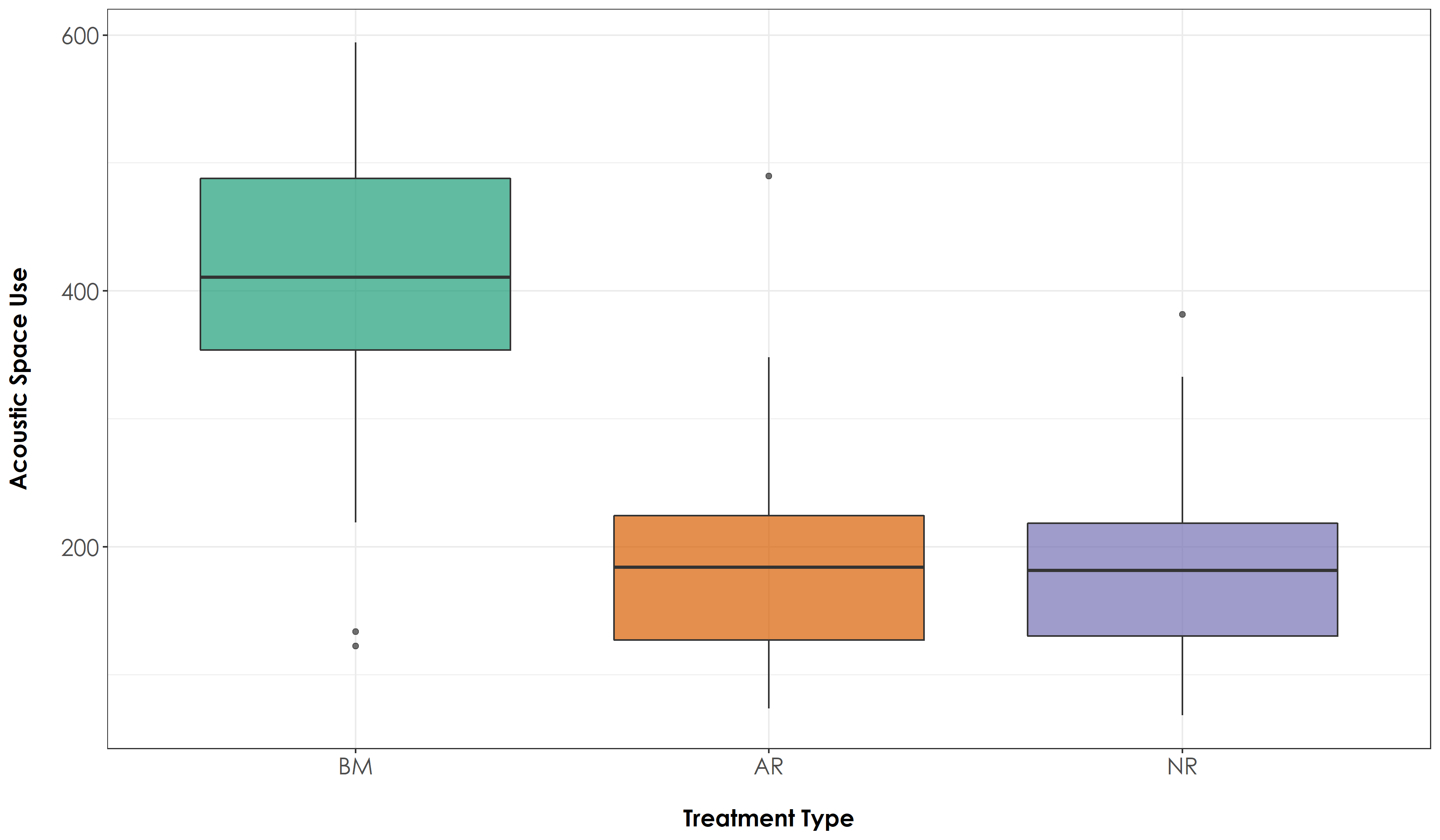
We now run generalized linear mixed models (GLMM) assuming gaussian errors to examine the effects of restoration type (benchmark, actively restored and passively restored) on acoustic space use, followed by TukeyHSD multiple comparisons tests of means.
# overall space use
glmm_allRestoration <- glmer(roundSpaceuse ~ Restoration.type + (1|siteCode) + (1|visit), data = modelDataAll, family = gaussian(link="identity"))

summary(glmm_allRestoration)
tukey_glmmAllRestoration <- summary(glht(glmm_allRestoration, linfct=mcp(Restoration.type ="Tukey")))
cld(tukey_glmmAllRestoration)

# The above result suggests a significant difference in acoustic space use between BM-AR and BM-NR sites, but no difference between AR and NR sites.

# diurnal
glmm_diurnalRestoration <- glmer(roundSpaceuse ~ Restoration.type + (1|siteCode) + (1|visit), data = modelDataDiurnal, family = gaussian(link="identity"))

summary(glmm_diurnalRestoration)
tukey_glmmDiurnalRestoration <- summary(glht(glmm_diurnalRestoration, linfct=mcp(Restoration.type ="Tukey")))
cld(tukey_glmmDiurnalRestoration)

# When we look at only the diurnal data, there is a significant difference in acoustic space use between BM-AR and BM-NR sites, but no difference between AR and NR sites.

# nocturnal data
glmm_nocturnalRestoration <- glmer(roundSpaceuse ~ Restoration.type + (1|siteCode) + (1|visit), data = modelDataNocturnal, family=gaussian(link="identity"))

summary(glmm_nocturnalRestoration)
tukey_glmmNocturnalRestoration <- summary(glht(glmm_nocturnalRestoration, linfct=mcp(Restoration.type ="Tukey")))
cld(tukey_glmmNocturnalRestoration)

# When we look at only the diurnal data, there is a significant difference in acoustic space use between BM-AR and BM-NR sites, but no difference between AR and NR sites.

# Plotting the above results

# reordering factors for plotting
modelDataAll$Restoration.type <- factor(modelDataAll$Restoration.type, levels = c("Benchmark", "Active", "Passive"))
# Add a custom set of colors
mycolors <- c(brewer.pal(name="Dark2", n = 3), brewer.pal(name="Paired", n = 3))

fig_glmm_allRest <- ggplot(modelDataAll, aes(Restoration.type, totSpaceuse, fill = Restoration.type)) +
  geom_boxplot(alpha=0.7) +
  scale_fill_manual("Treatment type",values=mycolors, labels=c("BM","AR","NR"))+
    theme_bw() +
    labs(x="\nTreatment Type",
       y="Acoustic Space Use\n") +
  scale_x_discrete(labels = c('BM','AR','NR')) +
    theme(axis.title = element_text(family = "Century Gothic",
      size = 14, face = "bold"),
        axis.text = element_text(family="Century Gothic",size = 14),
        legend.position = "none")

ggsave(fig_glmm_allRest, filename = "figs/fig_glmm_overallAcousticSpace.png", width=12, height=7, device = png(), units="in", dpi = 300);dev.off()

# reordering factors for plotting
modelDataDiurnal$Restoration.type <- factor(modelDataDiurnal$Restoration.type, levels = c("Benchmark", "Active", "Passive"))

fig_glmm_diurnalRest <- ggplot(modelDataDiurnal, aes(Restoration.type, totSpaceuse, group = Restoration.type, fill = Restoration.type)) +
 geom_boxplot(alpha = 0.7) +
  scale_fill_manual("Treatment type",values=mycolors, labels=c("BM","AR","NR")) +
    theme_bw() +
    labs(x="\nTreatment Type",
       y="Acoustic Space Use\n") +
  scale_x_discrete(labels = c('BM','AR','NR')) +
    theme(axis.title = element_text(family = "Century Gothic",
      size = 14, face = "bold"),
        axis.text = element_text(family="Century Gothic",size = 14),
        legend.position = "none")

ggsave(fig_glmm_diurnalRest, filename = "figs/fig_glmm_diurnalAcousticSpaceUse.png", width=12, height=7, device = png(), units="in", dpi = 300);dev.off()

# reordering factors for plotting
modelDataNocturnal$Restoration.type <- factor(modelDataNocturnal$Restoration.type, levels = c("Benchmark", "Active", "Passive"))

fig_glmm_nocturnalRest <- ggplot(modelDataNocturnal, aes(Restoration.type, totSpaceuse, group = Restoration.type, fill = Restoration.type)) +
  geom_boxplot(alpha = 0.7) +
  scale_fill_manual("Treatment type",values=mycolors, labels=c("BM","AR","NR")) +
    theme_bw() +
    labs(x="\nTreatment Type",
       y="Acoustic Space Use\n") +
  scale_x_discrete(labels = c('BM','AR','NR')) +
    theme(axis.title = element_text(family = "Century Gothic",
      size = 14, face = "bold"),
        axis.text = element_text(family="Century Gothic",size = 14),
        legend.position = "none")

ggsave(fig_glmm_nocturnalRest, filename = "figs/fig_glmm_nocturnalAcousticSpaceUse.png", width=12, height=7, device = png(), units="in", dpi = 300);dev.off()
Overall acoustic space use across treatment types. Analysis of ~4,128 hours of acoustic data across treatment types (for the 43 sites) revealed significant differences in ASU across BM-AR and BM-NR sites, with the highest estimate in BM sites (mean ± SD: 413 ± 103), followed by AR sites (mean ± SD: 188 ± 78) and NR sites (mean ± SD: 182 ± 66). In the above figure, BM = undisturbed benchmark rainforest sites, AR = Actively restored forest sites and NR = Naturally regenerating forest sites.
6.5 We now run generalized linear mixed models (GLMM) assuming gaussian errors and using log link functions to examine the effects of habitat (vegetation structure) on acoustic space use.
# overall space use
glmm_allVeg<- glmer(roundSpaceuse ~ PC1 + PC2 + (1|siteCode) + (1|visit), data = modelDataAll, family = gaussian(link="identity"))

summary(glmm_allVeg)
plot_model(glmm_allVeg, type="pred", terms=c("PC1","PC2"))
report::report(glmm_allVeg)

# We fitted a linear mixed model (estimated using REML and nloptwrap optimizer) to predict roundSpaceuse with PC1 and PC2 (formula: roundSpaceuse ~ PC1 + PC2). The model included siteCode and visit as random effects (formula: list(~1 | siteCode, ~1 | visit)). The model's total explanatory power is substantial (conditional R2 = 0.77) and the part related to the fixed effects alone (marginal R2) is of 0.10. The model's intercept, corresponding to PC1 = 0 and PC2 = 0, is at 294.12 (95% CI [254.39, 333.84], t(204) = 14.60, p < .001). Within this model:

#  - The effect of PC1 is statistically significant and negative (beta = -20.20, 95% CI [-29.35, -11.04], t(204) = -4.35, p < .001; Std. beta = -0.28, 95% CI [-0.41, -0.15])
#  - The effect of PC2 is statistically non-significant and negative (beta = -12.66, 95% CI [-26.83, 1.51], t(204) = -1.76, p = 0.080; Std. beta = -0.10, 95% CI [-0.22, 0.01])

# Standardized parameters were obtained by fitting the model on a standardized version of the dataset. 95% Confidence Intervals (CIs) and p-values were computed using the Wald approximation

# diurnal
glmm_diurnalVeg<- glmer(roundSpaceuse ~ PC1 + PC2 + (1|siteCode) + (1|visit), data = modelDataDiurnal, family = gaussian(link="identity"))

summary(glmm_diurnalVeg)
plot_model(glmm_diurnalVeg, type="pred", terms=c("PC2","PC1"))
report::report(glmm_diurnalVeg)

# We fitted a linear mixed model (estimated using REML and nloptwrap optimizer) to predict roundSpaceuse with PC1 and PC2 (formula: roundSpaceuse ~ PC1 + PC2). The model included siteCode and visit as random effects (formula: list(~1 | siteCode, ~1 | visit)). The model's explanatory power related to the fixed effects alone (marginal R2) is 0.26. The model's intercept, corresponding to PC1 = 0 and PC2 = 0, is at 145.60 (95% CI [122.30, 168.89], t(204) = 12.32, p < .001). Within this model:

#  - The effect of PC1 is statistically significant and negative (beta = -12.91, 95% CI [-18.99, -6.82], t(204) = -4.18, p < .001; Std. beta = -0.29, 95% CI [-0.43, -0.15])
#  - The effect of PC2 is statistically non-significant and negative (beta = -1.10, 95% CI [-10.62, 8.43], t(204) = -0.23, p = 0.821; Std. beta = -0.01, 95% CI [-0.14, 0.11])

# Standardized parameters were obtained by fitting the model on a standardized version of the dataset. 95% Confidence Intervals (CIs) and p-values were computed using the Wald approximation.

# nocturnal
glmm_nocturnalVeg<- glmer(roundSpaceuse ~ PC1 + PC2 + (1|siteCode) + (1|visit), data = modelDataNocturnal, family = gaussian(link="identity"))

summary(glmm_nocturnalVeg)
plot_model(glmm_nocturnalVeg, type="pred", terms=c("PC1","PC2"))
report::report(glmm_nocturnalVeg)

# We fitted a linear mixed model (estimated using REML and nloptwrap optimizer) to predict roundSpaceuse with PC1 and PC2 (formula: roundSpaceuse ~ PC1 + PC2). The model included siteCode and visit as random effects (formula: list(~1 | siteCode, ~1 | visit)). The model's total explanatory power is substantial (conditional R2 = 0.80) and the part related to the fixed effects alone (marginal R2) is of 0.05. The model's intercept, corresponding to PC1 = 0 and PC2 = 0, is at 134.62 (95% CI [110.39, 158.85], t(204) = 10.96, p < .001). Within this model:

#  - The effect of PC1 is statistically significant and negative (beta = -6.95, 95% CI [-12.04, -1.87], t(204) = -2.70, p = 0.008; Std. beta = -0.19, 95% CI [-0.32, -0.05])
#  - The effect of PC2 is statistically significant and negative (beta = -10.09, 95% CI [-17.89, -2.28], t(204) = -2.55, p = 0.012; Std. beta = -0.16, 95% CI [-0.28, -0.04])

# Standardized parameters were obtained by fitting the model on a standardized version of the dataset. 95% Confidence Intervals (CIs) and p-values were computed using the Wald approximation.
6.6 Main Text Figure 4
# Patchworking nmds and glmm for acoustic space use to create part a and b for Fig. 4
library(patchwork)

fig_glmm_ordinations <-
  wrap_plots(fig_glmm_allRest, fig_nmds,
    design = "AABBBB"
  ) +
  plot_annotation(
    tag_levels = "a",
    tag_prefix = "(",
    tag_suffix = ")"
  )

# Expand the width to avoid compression
ggsave(fig_glmm_ordinations, filename = "figs/fig04.png", width=20, height=7,device = png(), units="in", dpi = 300); dev.off()
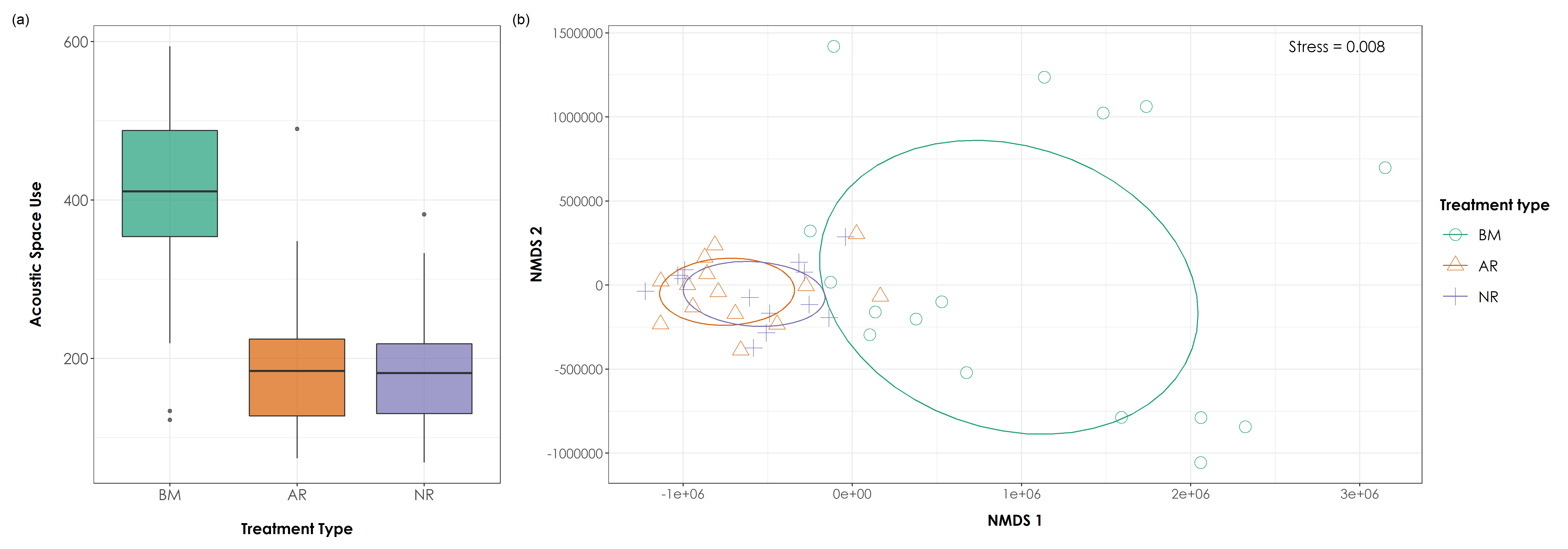
Acoustic space use across treatment types. (a) Analysis of ~4,128 hours of acoustic data across treatment types (for the 43 sites) revealed significant differences in ASU between BM-AR and BM-NR sites (Tukey HSD P < 0.05). ASU was the highest in BM sites (mean ± SD: 413 ± 103), followed by AR sites (mean ± SD: 188 ± 78) and NR sites (mean ± SD: 182 ± 66). (b) NMDS ordination of ASU (stress = 0.008) revealed a loose cluster of benchmark sites, while actively restored and naturally regenerating sites showed tight overlapping clusters. In the above figure, BM = undisturbed benchmark rainforest sites, AR = Actively restored forest sites, and NR = Naturally regenerating forest sites.