Section 11 Species relative abundances over time
In this script, we calculate species relative abundances over time by replicating a novel approach proposed by Gotelli et al. 2021 (who provides a methodological approach to calculate relative species abundances using historical museum records).
The assumption is that the level of the analysis is at the ‘historic-site’ and not the ‘modern-site’ (which essentially corresponds to multiple unique modern survey sites for every ‘historic-site’).
11.1 Load necessary libraries
library(dplyr)
library(stringr)
library(tidyverse)
library(scico)
library(RColorBrewer)
library(extrafont)
library(sf)
library(raster)
library(lattice)
library(data.table)
library(ggrepel)
library(report)
library(lme4)
library(glmmTMB)
library(multcomp)
library(ggstatsplot)
library(paletteer)
library(ggpubr)
library(goeveg)
library(sjPlot)
library(patchwork)

# source custom functions
source("code/02_relative-species-abundance-functions.R")
11.2 Load list of resurvey locations
We will load the list of sites across which a modern resurvey was carried out, along with elevation rasters.
# load list of resurvey locations and add elevation as a variable
# remove the modern resurvey locations only (ie. ASFQ)
sites <- read.csv("data/list-of-resurvey-locations.csv")
sites <- sites[-c(1:50), ]

# convert to sf object and transform
sites <- st_as_sf(sites, coords = c("longitude", "latitude")) %>%
  `st_crs<-`(4326) %>%
  st_transform(32643)

# add elevation raster
alt <- raster::raster("data/elevation/alt") # this layer is not added to github as a result of its large size and can be downloaded from SRTM (Farr et al. (2007))

# extract values from that raster (note: transformation of coordinate system)
elev <- raster::extract(alt, sites)
sites <- cbind(sites, elev)
11.3 Calibrating historical data to modern survey data for relative abundance calculations
To ensure that museum specimens and associated observations are comparable with field associated surveys, since they are both independent sources of information, we calibrate them to understand if they are comparable in the first place.
## read in historical occurrence data
hist_occ <- read.csv("data/historical-occurrence-data.csv")

## applying filters:
# include only data until 1950
hist_occ <- hist_occ %>%
  filter(year <= 1950)

# total species count across historical data
spp_count <- hist_occ %>%
  group_by(scientific_name, common_name) %>%
  count() # total of 179 species

sppMinThree <- spp_count %>%
  filter(n >= 3) # total of 92 species

## read in modern occurrence data
mod_occ <- read.csv("data/modern-occurrence-data.csv") %>%
  filter(!is.na(historical_site_code)) # 2301 observations of 103 bird species

# ensure the data is comparable with historical data
mod_occ <- mod_occ %>%
  filter(!is.na(species_code)) %>%
  filter(common_name %in% hist_occ$common_name) %>%
  filter(historical_site_code %in% hist_occ$historical_site_code)

# total species count across historical data
mod_spp_count <- mod_occ %>%
  group_by(common_name) %>%
  count()

## group by scientific name and modern site code
mod_occ <- mod_occ %>%
  filter(!is.na(common_name)) %>%
  group_by(common_name, modern_site_code) %>%
  summarise("2021" = sum(number))

## left join the sites dataframe
mod_occ <- left_join(mod_occ, sites, by = c("modern_site_code" = "modern_site_code")) %>%
  filter(!is.na(common_name)) %>%
  replace(is.na(.), 0)

# calculate total count of historical data at each site
# here we pool all historical data from 1850-1950
hist_occ_tot <- hist_occ %>%
  group_by(common_name, historical_site_code) %>%
  count() %>%
  summarise("historical" = sum(n))

# left join the sites dataframe
hist_occ_tot <- left_join(hist_occ_tot, sites, by = c("historical_site_code" = "historical_site_code")) %>%
  filter(!is.na(common_name)) %>%
  replace(is.na(.), 0)

# we remove modern site_code and get only distinct rows
unique_hist <- hist_occ_tot[, c(1, 2, 3)] %>%
  group_by(common_name, historical_site_code) %>%
  distinct() %>%
  group_by(common_name) %>%
  summarise("relAbundHist" = sum(historical))

# we remove modern site_code and get only distinct rows
unique_mod <- mod_occ[, c(1, 3, 5)] %>%
  group_by(common_name, historical_site_code) %>%
  distinct() %>%
  group_by(common_name) %>%
  summarise("relAbund2021" = sum(`2021`))

# join historical and modern dataframes
hist_mod <- full_join(unique_hist, unique_mod) %>%
  replace_na(list(
    relAbundHist = 0,
    relAbund2021 = 0
  ))

# apply dirichlet distribution to the historical data
# choosing 1850-1900 data first
dat <- tibble::deframe(hist_mod[, 1:2])

relAbunHist <- dirch_stats(dat) %>%
  dplyr::select(species, bayes_mean) %>%
  rename(., bayes_mean_hist = bayes_mean)

# apply dirichlet distribution to the modern survey
dat <- tibble::deframe(hist_mod[, c(1, 3)]) ## choosing modern data

relAbun2021 <- dirch_stats(dat) %>%
  dplyr::select(species, bayes_mean) %>%
  rename(., bayes_mean_2021 = bayes_mean)

# for calibration
### join the relative abundance datasets together
relAbunCalib <- full_join(relAbunHist, relAbun2021) %>%
  arrange(species) %>%
  rename(., "historical" = "bayes_mean_hist") %>%
  rename(., "modern" = "bayes_mean_2021") %>%
  rename(., common_name = species)

# regressing 1850-1950 data vs. 2021
fig_hist_v_mod_rel <- ggplot(data = relAbunCalib, aes(x = modern, y = historical)) +
  scale_y_log10() +
  geom_abline(slope = 1, intercept = 0, linetype = "dashed") +
  scale_x_log10() +
  labs(
    y = "Historical Relative abundance",
    x = "Modern Relative abundance"
  ) +
  geom_point(shape = 21, colour = "black", fill = "white", size = 2, stroke = 1) +
  geom_smooth(method = "lm", se = TRUE, fullrange = FALSE, level = 0.95, linetype = "solid") +
  stat_regline_equation(aes(label = ..rr.label..)) +
  # geom_text_repel(aes(label = common_name),family = "Century Gothic", fontface = "italic") +
  theme_bw() +
  theme(
    axis.text = element_text(family = "Century Gothic", size = 13),
    legend.title = element_text(family = "Century Gothic"),
    legend.text = element_text(family = "Century Gothic"),
    text = element_text(family = "Century Gothic", size = 25)
  )

ggsave(fig_hist_v_mod_rel, filename = "figs/fig_historical_vs_modern_relAbun.png", width = 15, height = 10, device = png(), units = "in", dpi = 300)
dev.off()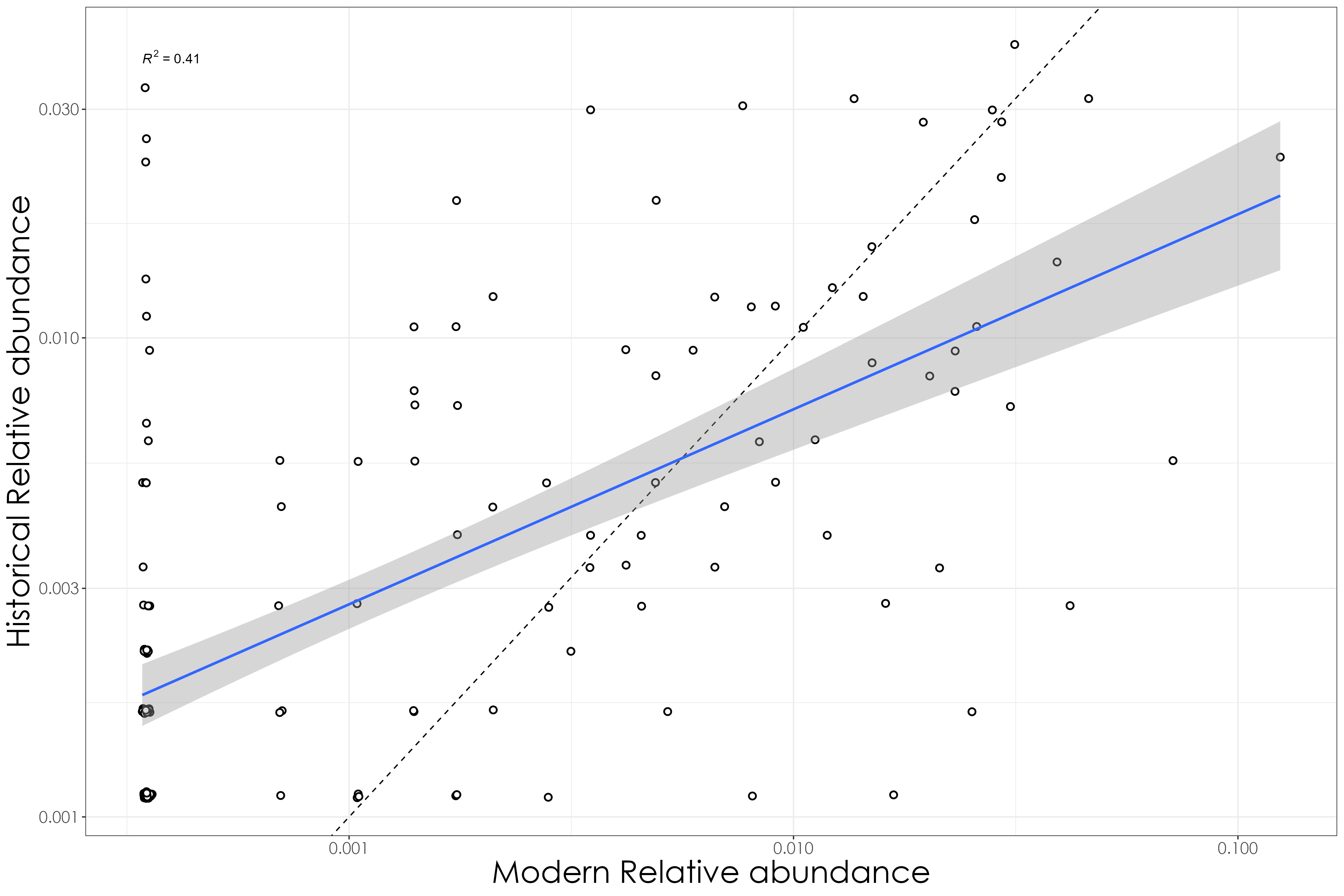
11.4 Calculating species relative abundance for the historical data (1850-1900 and 1900-1950)
## read in historical occurrence data
hist_occ <- read.csv("data/historical-occurrence-data.csv")

## applying filters:
# a: include only data until 1950
hist_occ <- hist_occ %>%
  filter(year <= 1950)

# b: a second filter includes only those species that had a minimum count of atleast three specimens and occurred across atleast two unique historical survey locations

# total species count across historical data
spp_count <- hist_occ %>%
  group_by(common_name) %>%
  count() # total of 179 species

sppMinThree <- spp_count %>%
  filter(n >= 3)

# please note, we include ~four species that were collected from a single historical location Apus melba, Apus melba, Brachypodius priocephalus, Phylloscopus tytleri, Picus chlorolophus

# filter historical data
hist_occ <- hist_occ %>%
  filter(common_name %in% sppMinThree$common_name)

### pre-1900
hist_occ_pre1900 <- hist_occ %>%
  filter(year <= 1900)

# calculate total count of historical data at each site
hist_occ_pre1900 <- hist_occ_pre1900 %>%
  group_by(common_name, historical_site_code) %>%
  count() %>%
  summarise("1850-1900" = sum(n))

# left join the sites dataframe
hist_occ_pre1900 <- left_join(hist_occ_pre1900, sites, by = c("historical_site_code" = "historical_site_code")) %>%
  filter(!is.na(common_name)) %>%
  replace(is.na(.), 0)

## 1900-1950 data
hist_occ_1900_1950 <- hist_occ %>%
  filter(year > 1900 & year <= 1950)

# calculate total count of historical data at each site
hist_occ_1900_1950 <- hist_occ_1900_1950 %>%
  group_by(common_name, historical_site_code) %>%
  count() %>%
  summarise("1900-1950" = sum(n))

# left join the sites dataframe
hist_occ_1900_1950 <- left_join(hist_occ_1900_1950, sites, by = c("historical_site_code" = "historical_site_code")) %>%
  filter(!is.na(common_name)) %>%
  replace(is.na(.), 0)
11.5 Load the modern occurrence data
For the modern occurrence data, we only keep species that were recorded historically to avoid artificial increases in relative abundance due to the method of collection.
mod_occ <- read.csv("data/modern-occurrence-data.csv") %>%
  filter(!is.na(historical_site_code)) # 2301 observations of 103 bird species

# ensure the data is comparable with historical data
mod_occ <- mod_occ %>%
  filter(!is.na(species_code)) %>%
  filter(common_name %in% hist_occ$common_name) %>%
  filter(historical_site_code %in% hist_occ$historical_site_code)

# total species count across historical data
mod_spp_count <- mod_occ %>%
  group_by(common_name) %>%
  count() # total of 63 spp

## group by scientific name and modern site code
mod_occ <- mod_occ %>%
  filter(!is.na(common_name)) %>%
  group_by(common_name, modern_site_code) %>%
  summarise("2021" = sum(number))

## left join the sites dataframe
mod_occ <- left_join(mod_occ, sites, by = c("modern_site_code" = "modern_site_code")) %>%
  filter(!is.na(common_name)) %>%
  replace(is.na(.), 0)
11.6 Calculate dirichlet distributions of relative abundance
Here, we will functions from Gotelli et al. 2023 to calculate relative species abundances between historic and modern periods.
# note: the level of the analysis is at the 'historic-site' and not the 'modern-site' (which essentially corresponds to two or three unique sites for every 'historic-site')
# to ensure that the analysis is consistent, we sum abundances across the modern sites corresponding to each historic site
# However, our analysis calculates relative species abundances for the give time period rather than by site + time-period

# we remove modern site_code and get only distinct rows
unique_hist_pre1900 <- hist_occ_pre1900[, c(1, 2, 3)] %>%
  group_by(common_name, historical_site_code) %>%
  distinct() %>%
  group_by(common_name) %>%
  summarise("relAbund1850" = sum(`1850-1900`))

# we remove modern site_code and get only distinct rows
unique_hist_1900_1950 <- hist_occ_1900_1950[, c(1, 2, 3)] %>%
  group_by(common_name, historical_site_code) %>%
  distinct() %>%
  group_by(common_name) %>%
  summarise("relAbund1900" = sum(`1900-1950`))

# we remove modern site_code and get only distinct rows
unique_mod <- mod_occ[, c(1, 3, 5)] %>%
  group_by(common_name, historical_site_code) %>%
  distinct() %>%
  group_by(common_name) %>%
  summarise("relAbund2021" = sum(`2021`))

hist_mod <- full_join(
  unique_hist_pre1900,
  unique_hist_1900_1950
) %>%
  full_join(., unique_mod) %>%
  replace_na(list(
    relAbund1850 = 0,
    relAbund1900 = 0,
    relAbund2021 = 0
  ))

# apply dirichlet distribution to the historical data
# choosing 1850-1900 data first
dat <- tibble::deframe(hist_mod[, 1:2])

relAbun1850 <- dirch_stats(dat) %>%
  dplyr::select(species, bayes_mean) %>%
  rename(., bayes_mean_1850 = bayes_mean)

# choosing 1900-1950 data
dat <- tibble::deframe(hist_mod[, c(1, 3)])

relAbun1900 <- dirch_stats(dat) %>%
  dplyr::select(species, bayes_mean) %>%
  rename(., bayes_mean_1900 = bayes_mean)

# apply dirichlet distribution to the modern survey
dat <- tibble::deframe(hist_mod[, c(1, 4)]) ## choosing modern data

relAbun2021 <- dirch_stats(dat) %>%
  dplyr::select(species, bayes_mean) %>%
  rename(., bayes_mean_2021 = bayes_mean)

### join the relative abundance datasets together
relAbun <- full_join(relAbun1850, relAbun1900) %>%
  full_join(., relAbun2021) %>%
  arrange(species) %>%
  rename(., `1850-1900` = "bayes_mean_1850") %>%
  rename(., `1900-1950` = "bayes_mean_1900") %>%
  rename(., `2021` = "bayes_mean_2021") %>%
  rename(., common_name = species)
11.7 Boxplot visualization of overall relative abundance across time periods
data_for_boxplot <- relAbun %>%
  dplyr::select(-common_name) %>%
  pivot_longer(everything())

fig_relAbun_over_time <- ggbetweenstats(
  data = data_for_boxplot,
  x = name,
  y = value,
  xlab = "Time Period",
  ylab = "Relative Abundance",
  title = "Relative abundance by time period",
  violin.args = list(width = 0),
  pairwise.comparisons = T
) +
  scale_y_log10() +
  # scale_color_manual(values = c("#9EB0FFFF", "#122C39FF","#D5857DFF")) +
  theme(
    plot.title = element_text(
      family = "Century Gothic",
      size = 18, face = "bold"
    ),
    axis.title = element_text(
      family = "Century Gothic",
      size = 16, face = "bold"
    ),
    axis.text = element_text(
      family = "Century Gothic",
      size = 14
    ),
    plot.subtitle = element_text(
      family = "Century Gothic",
      size = 14,
      face = "bold",
      color = "#1b2838"
    )
  )

ggsave(fig_relAbun_over_time, filename = "figs/fig_relAbun_landscapeLevel.png", width = 15, height = 10, device = png(), units = "in", dpi = 300)
dev.off()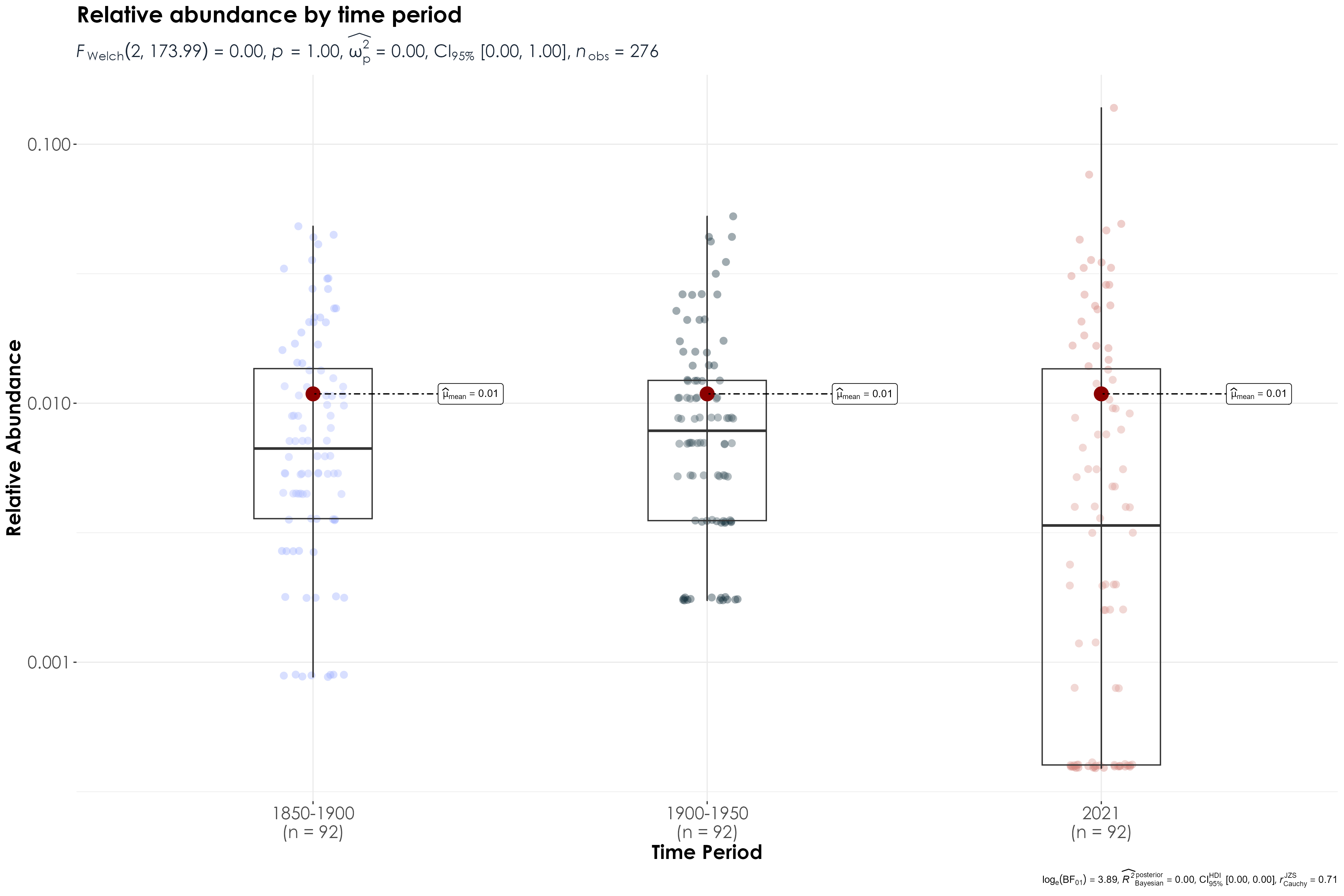
11.8 Species relative abundances at the site-level
We now recalculate species relative abundances at the site-level, which will be used for downstream comparisons with change in land cover and climate at a given site.
# 1850-1900 data
# we remove modern site_code and get only distinct rows
hist_pre1900 <- hist_occ_pre1900[, c(1:3)] %>%
distinct(.)
# 1900-1950 data
# we remove modern site_code and get only distinct rows
hist_1900_1950 <- hist_occ_1900_1950[, c(1:3)] %>%
distinct(.)
## modern resurvey
## analysis is being done at the level of the historical site code
mod_site_level <- mod_occ[, c(1, 3, 5)] %>%
group_by(common_name, historical_site_code) %>%
mutate("2021" = sum(`2021`)) %>%
distinct(.)
## join data frames together
site_level_relAbun <- full_join(
hist_pre1900,
hist_1900_1950
) %>%
full_join(., mod_site_level) %>%
replace_na(list(
`1850-1900` = 0,
`1900-1950` = 0,
`2021` = 0
)) %>%
ungroup() %>%
complete(common_name, historical_site_code,
fill = list(
`1850-1900` = 0,
`1900-1950` = 0,
`2021` = 0
)
)
## site-level relative abundance for 1850-1900 data
relSpAbund_1850_1900 <- c()
for (i in 1:length(unique(site_level_relAbun$historical_site_code))) {
# for every unique historical site
a <- site_level_relAbun %>%
filter(historical_site_code == unique(site_level_relAbun$historical_site_code)[i])
# subset historical data
b <- tibble::deframe(a[, c(1, 3)]) ## choosing 1850-1900 data
loc <- unique(site_level_relAbun$historical_site_code)[i] # what's the site_code?
## historical relative abundance
relSpAbund_1850_1900[[i]] <- dirch_stats(b) %>%
dplyr::select(species, bayes_mean)
old_varname <- c("species", "bayes_mean")
new_varname <- c("common_name", paste(loc, "_", "1850", sep = ""))
relSpAbund_1850_1900[[i]] <- relSpAbund_1850_1900[[i]] %>%
data.table::setnames(old = old_varname, new = new_varname)
names(relSpAbund_1850_1900)[i] <- loc
}
# save object but full_join across lists
relSpAbund_1850_1900 <- relSpAbund_1850_1900 %>%
reduce(.f = full_join)
## site-level relative abundance for 1900-1950 data
relSpAbund_1900_1950 <- c()
for (i in 1:length(unique(site_level_relAbun$historical_site_code))) {
# for every unique historical site
a <- site_level_relAbun %>%
filter(historical_site_code == unique(site_level_relAbun$historical_site_code)[i])
# subset historical data
b <- tibble::deframe(a[, c(1, 4)]) ## choosing 1900-1950 data
loc <- unique(site_level_relAbun$historical_site_code)[i] # what's the site_code?
## historical relative abundance
relSpAbund_1900_1950[[i]] <- dirch_stats(b) %>%
dplyr::select(species, bayes_mean)
old_varname <- c("species", "bayes_mean")
new_varname <- c("common_name", paste(loc, "_", "1900", sep = ""))
relSpAbund_1900_1950[[i]] <- relSpAbund_1900_1950[[i]] %>%
data.table::setnames(old = old_varname, new = new_varname)
names(relSpAbund_1900_1950)[i] <- loc
}
# save object but full_join across lists
relSpAbund_1900_1950 <- relSpAbund_1900_1950 %>%
reduce(.f = full_join)
# modern resurvey relative abundance - site level
relSpAbund_2021 <- c()
for (i in 1:length(unique(site_level_relAbun$historical_site_code))) {
a <- site_level_relAbun %>%
filter(historical_site_code == unique(site_level_relAbun$historical_site_code)[i])
b <- tibble::deframe(a[, c(1, 5)]) ## choosing modern data
loc <- unique(site_level_relAbun$historical_site_code)[i] # what's the site_code?
relSpAbund_2021[[i]] <- dirch_stats(b) %>%
dplyr::select(species, bayes_mean)
old_varname <- c("species", "bayes_mean")
new_varname <- c("common_name", paste(loc, "_", "2021", sep = ""))
relSpAbund_2021[[i]] <- relSpAbund_2021[[i]] %>%
data.table::setnames(old = old_varname, new = new_varname)
names(relSpAbund_2021)[i] <- loc
}
# save object but full_join across lists
relSpAbund_2021 <- relSpAbund_2021 %>%
reduce(.f = full_join)
## join all the datasets together
relSpAbund_by_site <- full_join(
relSpAbund_1850_1900,
relSpAbund_1900_1950
) %>%
full_join(., relSpAbund_2021) %>%
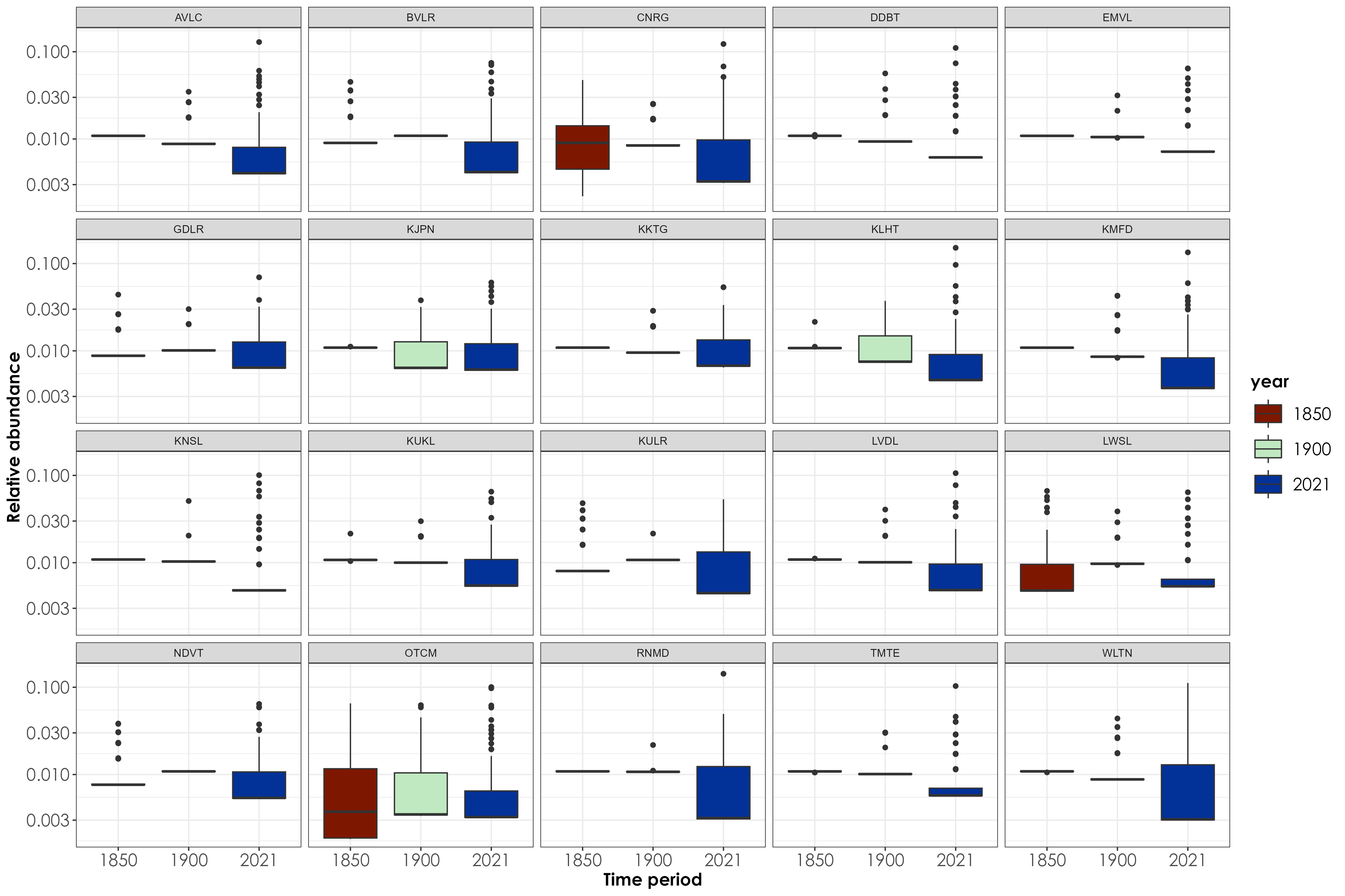
arrange(common_name)11.9 Visualizing differences in relative abundance over time at the site level
## preparing dataframe for visualization
relSpAbund <- relSpAbund_by_site %>%
  pivot_longer(!common_name, names_to = "site_year", values_to = "relAbundance") %>%
  separate(site_year, into = c("site", "year"), sep = "_")

## Please note: for the sake of downstream analysis, we have renamed 1850-1900 as 1850. In other words, each year - except for 2021 represents a 50 year time period.

fig_relAbun_siteLevel <- relSpAbund %>%
  dplyr::select(-common_name) %>%
  ggplot(aes(
    x = year, y = relAbundance,
    fill = year
  )) +
  geom_boxplot() +
  scale_y_log10() +
  facet_wrap(~site) +
  xlab("Time period") +
  ylab("Relative abundance") +
  scale_fill_scico_d(palette = "roma") +
  theme_bw() +
  theme(
    axis.title = element_text(
      family = "Century Gothic",
      size = 14, face = "bold"
    ),
    axis.text = element_text(family = "Century Gothic", size = 14),
    legend.title = element_text(
      family = "Century Gothic",
      size = 14, face = "bold"
    ),
    legend.key.size = unit(1, "cm"),
    legend.text = element_text(family = "Century Gothic", size = 14)
  )

ggsave(fig_relAbun_siteLevel, filename = "figs/fig_relAbun_siteLevel.png", width = 15, height = 10, device = png(), units = "in", dpi = 300)
dev.off()