Section 7 Hierarchical model approach
Here we want to evaluate the use of another approach for a hierarchical model of estimation of counts. First, we fit a dynamic autoregressive model to estimate stochastic counts that can be compared to conventional approaches (e.g., -mixture models). We can use this autoregressive model also to estimate the same latent counts from the acoustic detections data as observation process, including an extra parameter of scaling the acoustic activity (e.g., one individual singing more than a 1:1 relationship).
We try this option first with a single species in a single site. However, this can be further extrapolated to use multispecies models, from abundant species in the community to estimate parameters of rare ones (sharing some characteristics), such as Beta N-Mixture and Normal N-Mixture .
7.2 Loading and exploring data
Let’s load the file used in 01_data-comparability.Rmd script.
acous_count <- read_csv("results/pooled_pointCount_acoustic_data.csv")

acous_count |> # names()
  group_by(common_name, data_type, site_name) |>
  count() #|> View() # use filter in RStudio
Let’s work on the species-site combination of more data: Ovenbird in Marsh-Billings-Rockefeller NHP.
acous_count_filt <- acous_count |>
  filter(common_name %in% c(
    #"American Crow","American Robin","Black-and-white Warbler","Black-capped Chickadee","Black-throated Blue Warbler","Black-throated Green Warbler","Blackburnian Warbler","Blue Jay","Blue-headed Vireo","Brown Creeper","Eastern Wood-Pewee","Golden-crowned Kinglet","Hermit Thrush","Northern Parula",

                            "Ovenbird"

                            #,"Pine Warbler","Red-breasted Nuthatch","Red-eyed Vireo","Scarlet Tanager","Winter Wren","Yellow-bellied Sapsucker","Yellow-rumped Warbler"
                            ),
    site_name == "Marsh-Billings-Rockefeller NHP")
table(acous_count_filt$common_name, acous_count_filt$data_type)
The package naniar allow to see a good summar of NAs per column
How to reconcile time of detection of each record?
While the point_count data include the observation_time variable, this information for the acoustic_data seems to be at the begin_clock_time variable. Let’s adjust this with the function coalesce from dplyr in tidyverse. Then, we can consolidate the “initial temporal window” per visit in each site_id with the detection time.
acoust_count_summary <- acous_count_filt |>
  # dummy column to unify time of detection either by count or
  mutate(detection_time = coalesce(observation_time, begin_clock_time)) |>
  # initial temporal window
  group_by(site_id, date, visit_number) |>
  mutate(time_window = min(hms::as_hms(detection_time), na.rm = TRUE),
         time_window = hms::as_hms(time_window)) |>
  # First summarization to extract sum of counts per point count and number of detections
  group_by(site_name, site_id, date, visit_number, common_name, data_type, time_window, detection_time) |>
  summarise(abundance = sum(abundance, na.rm = TRUE),
         acous_detections = n()) |>
  # Second summarization to count number of detections and extract overall counts
  group_by(site_name, site_id, date, visit_number, common_name, time_window) |>
  summarise(counts = sum(abundance, na.rm = TRUE),
         acous_detections = sum(acous_detections)) |>
  as.data.frame()

acoust_count_summary$DateTime <- as.POSIXct(paste(acoust_count_summary$date, acoust_count_summary$time_window), format = "%Y-%m-%d %H:%M:%S")

acoust_count_summary$Time_window <- floor_date(acoust_count_summary$DateTime, "10 mins")

str(acoust_count_summary)
And we can generate the figures. This are similar to my previous attempt, but including some days or point counts discarded by Vijay due to species richness.
7.2.1 Figures of the data
Time series of the counts
ggplot(acoust_count_summary,
       aes(x = Time_window, y = counts, color = site_name)) +
  geom_segment(aes(y = 0, yend = counts), alpha = 0.3) +
  geom_point(alpha = 0.6) +
  facet_wrap(~common_name, ncol = 3) +
  labs(x = "Time",
       y = "Number of individuals counted in a 10-minute point count",
       color = "Site")+
  scale_color_manual(values=met.brewer("Homer2", 4))+
  theme_minimal()+
  theme(legend.position = "bottom")
#ggsave(filename = "figs/counts-by-time-continuous.jpg", width = 10, height = 10, units = "in", dpi = 300)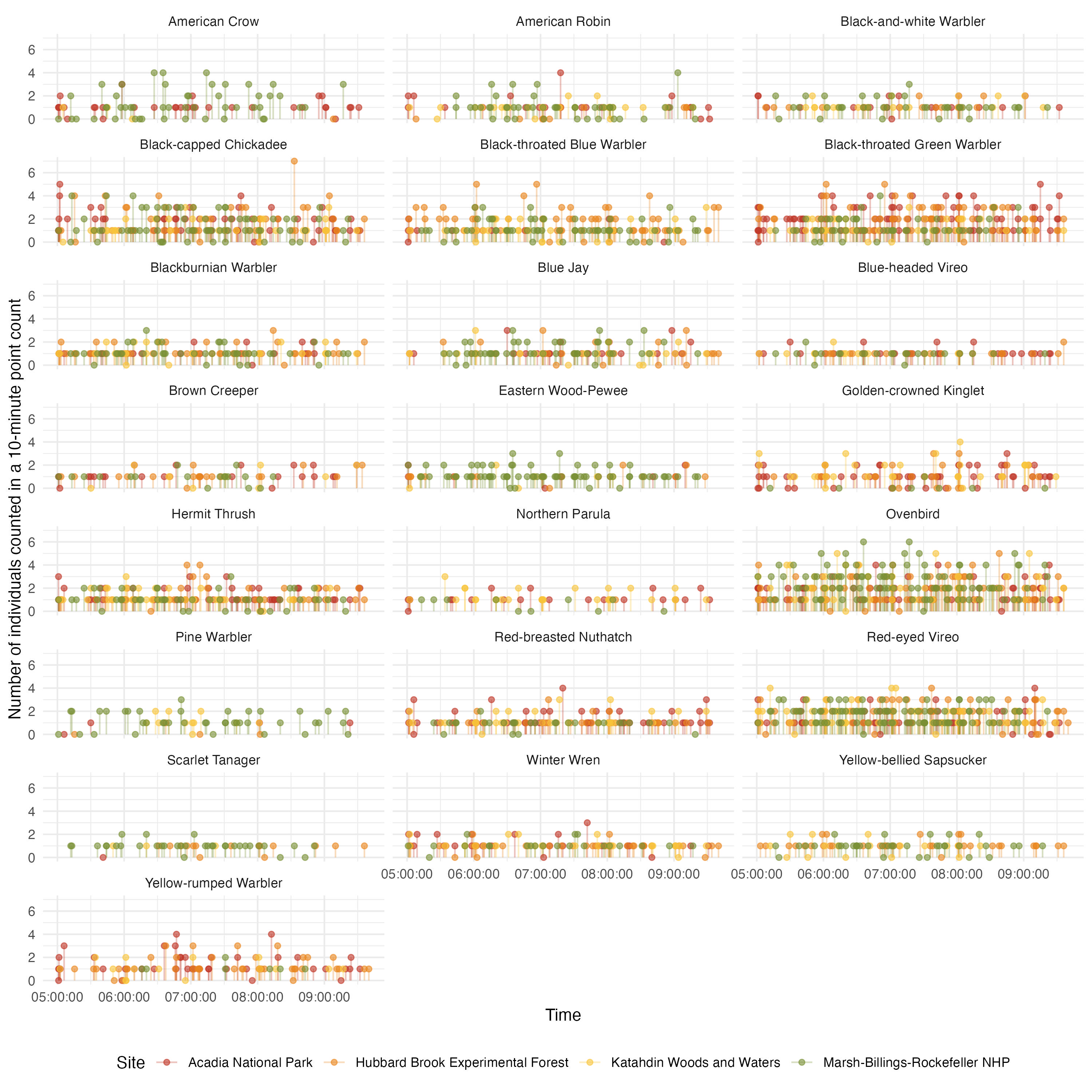
Time series of acoustic detections
ggplot(acoust_count_summary,
       aes(x = Time_window, y = acous_detections, color = site_name)) +
  geom_segment(aes(y = 0, yend = acous_detections), alpha = 0.3) +
  geom_point(alpha = 0.6) +
  facet_wrap(~common_name, ncol = 3, scales = "free_y") +
  labs(x = "Time",
       y = "Number of acoustic detections in a 10-minute recording",
       color = "Site")+
  scale_color_manual(values=met.brewer("Homer2", 4))+
  theme_minimal()+
  theme(legend.position = "bottom")
#ggsave(filename = "figs/acou_det-by-time-continuous.jpg", width = 10, height = 10, units = "in", dpi = 300)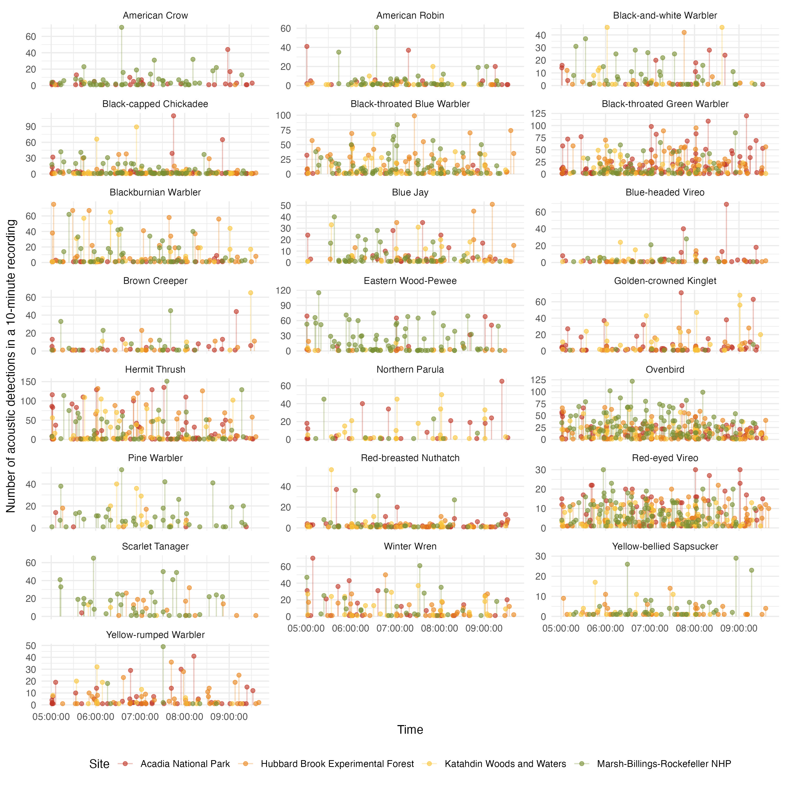
This summary dataset also allow to see the potential effect of phenology. We can see the two years independently
acoust_count_summary |>
  mutate(year = year(date)) |>
  filter(year == 2022) |>
  ggplot(aes(x = Time_window, y = counts, color = site_name))+
  geom_segment(aes(y = 0, yend = counts), alpha = 0.3) +
  geom_point(alpha = 0.6) +
  facet_wrap(~common_name, ncol = 3) +
  labs(x = "Date-Time of survey (2022)",
       y = "Number of individuals counted in a 10-minute point count",
       color = "Site")+
  scale_color_manual(values=met.brewer("Homer2", 4))+
  theme_minimal()+
  theme(legend.position = "bottom")
#ggsave(filename = "figs/counts-by-date_2022.jpg", width = 10, height = 10, units = "in", dpi = 300)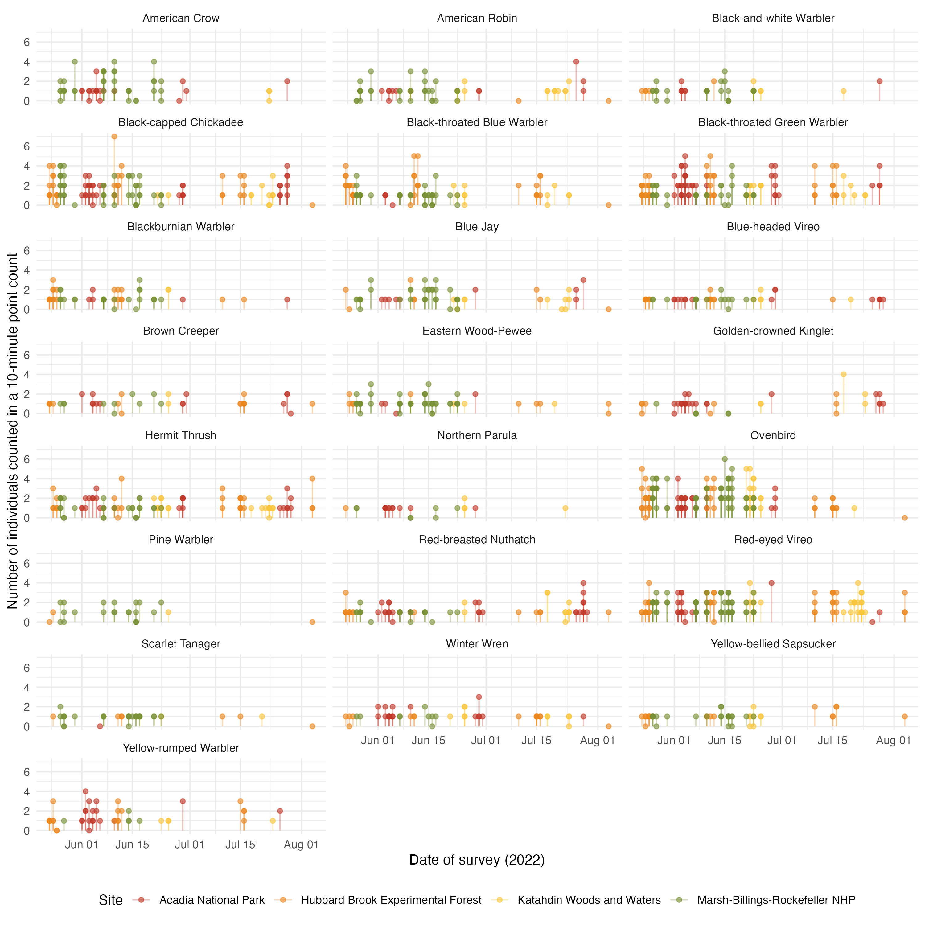
acoust_count_summary |>
  mutate(year = year(date)) |>
  filter(year == 2022) |>
  ggplot(aes(x = Time_window, y = acous_detections, color = site_name))+
  geom_segment(aes(y = 0, yend = acous_detections), alpha = 0.3) +
  geom_point(alpha = 0.6) +
  facet_wrap(~common_name, ncol = 3, scales = "free_y") +
  labs(x = "Date-Time of survey (2022)",
       y = "Number of acoustic detections in a 10-minute recording",
       color = "Site")+
  scale_color_manual(values=met.brewer("Homer2", 4))+
  theme_minimal()+
  theme(legend.position = "bottom")
#ggsave(filename = "figs/acou_det-by-date_2022.jpg", width = 10, height = 10, units = "in", dpi = 300)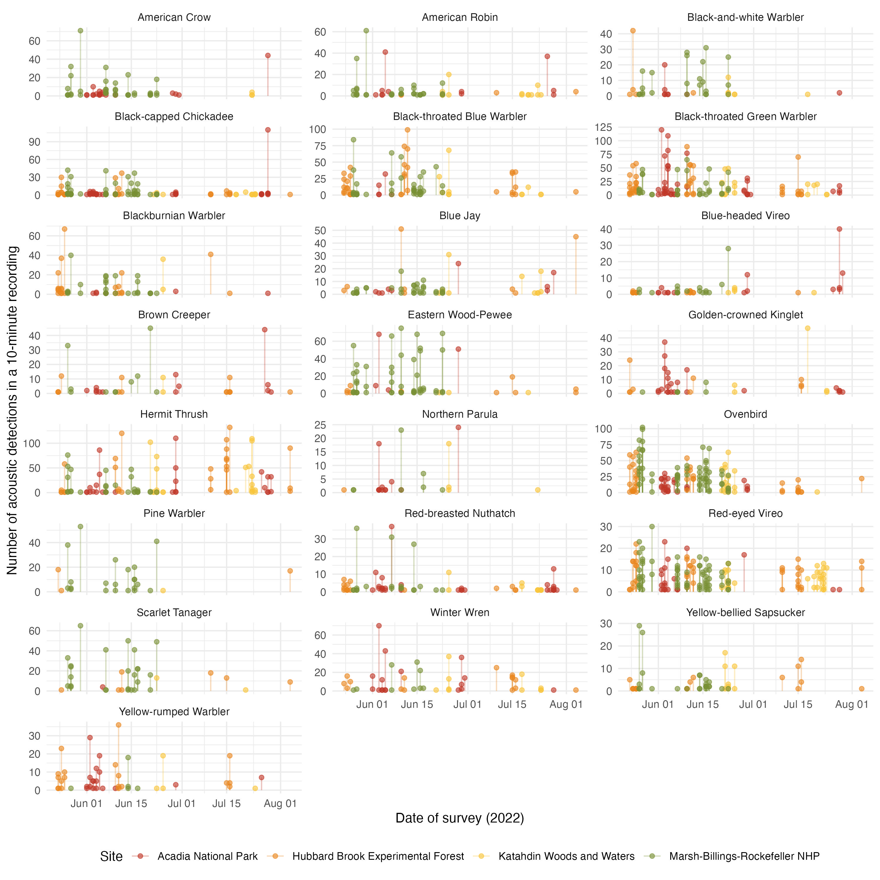
And for 2023:
acoust_count_summary |>
  mutate(year = year(date)) |>
  filter(year == 2023) |>
  ggplot(aes(x = DateTime, y = counts, color = site_name))+
  geom_segment(aes(y = 0, yend = counts), alpha = 0.3) +
  geom_point(alpha = 0.6) +
  facet_wrap(~common_name, ncol = 3) +
  labs(x = "Date of survey (2023)",
       y = "Number of individuals counted in a 10-minute point count",
       color = "Site")+
  scale_color_manual(values=met.brewer("Homer2", 4))+
  theme_minimal()+
  theme(legend.position = "bottom")
#ggsave(filename = "figs/counts-by-date_2023.jpg", width = 10, height = 10, units = "in", dpi = 300)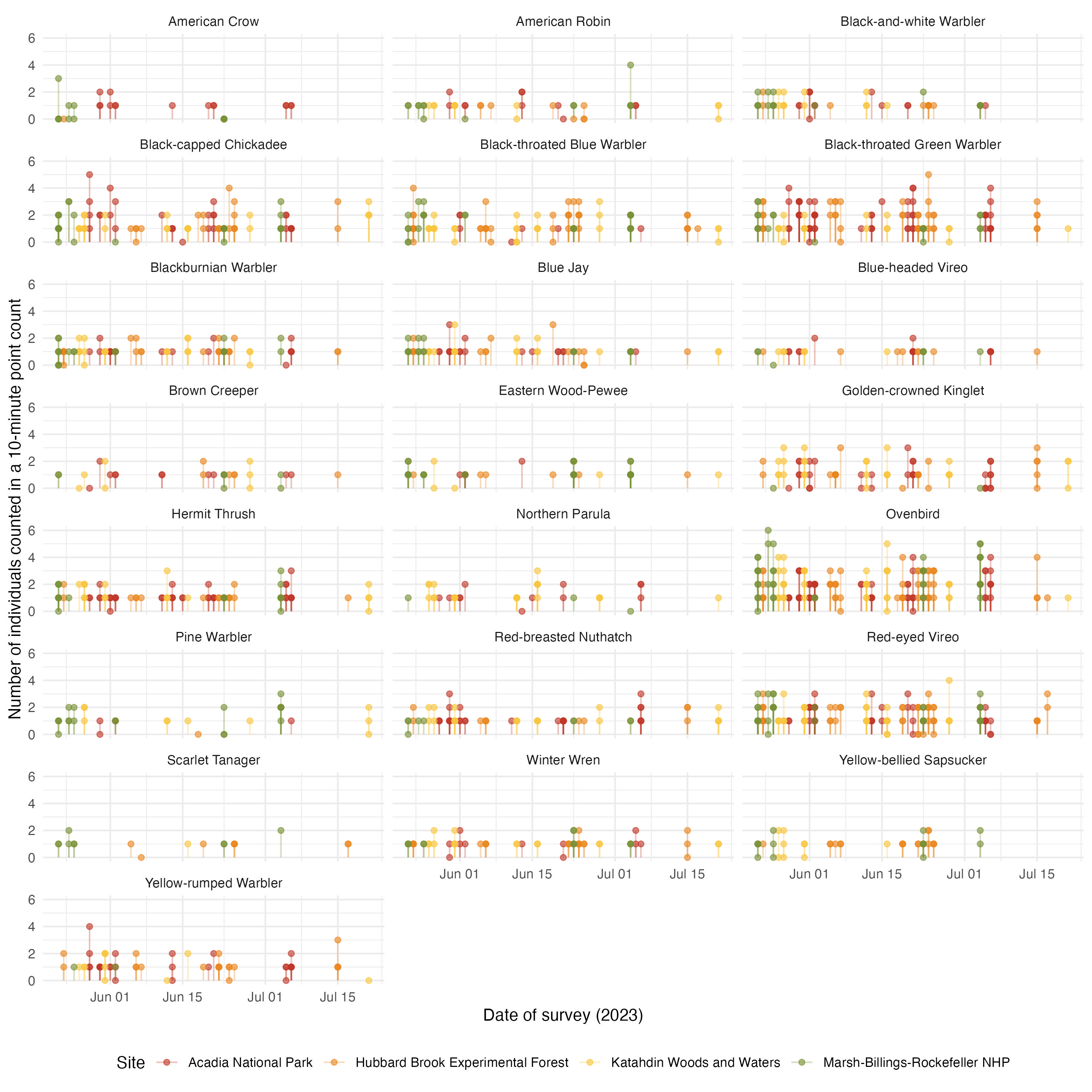
acoust_count_summary |>
  mutate(year = year(date)) |>
  filter(year == 2023) |>
  ggplot(aes(x = DateTime, y = acous_detections, color = site_name))+
  geom_segment(aes(y = 0, yend = acous_detections), alpha = 0.3) +
  geom_point(alpha = 0.6) +
  facet_wrap(~common_name, ncol = 3, scales = "free_y") +
  labs(x = "Date of survey (2023)",
       y = "Number of acoustic detections in a 10-minute recording",
       color = "Site")+
  scale_color_manual(values=met.brewer("Homer2", 4))+
  theme_minimal()+
  theme(legend.position = "bottom")
#ggsave(filename = "figs/acou_det-by-date_2023.jpg", width = 10, height = 10, units = "in", dpi = 300)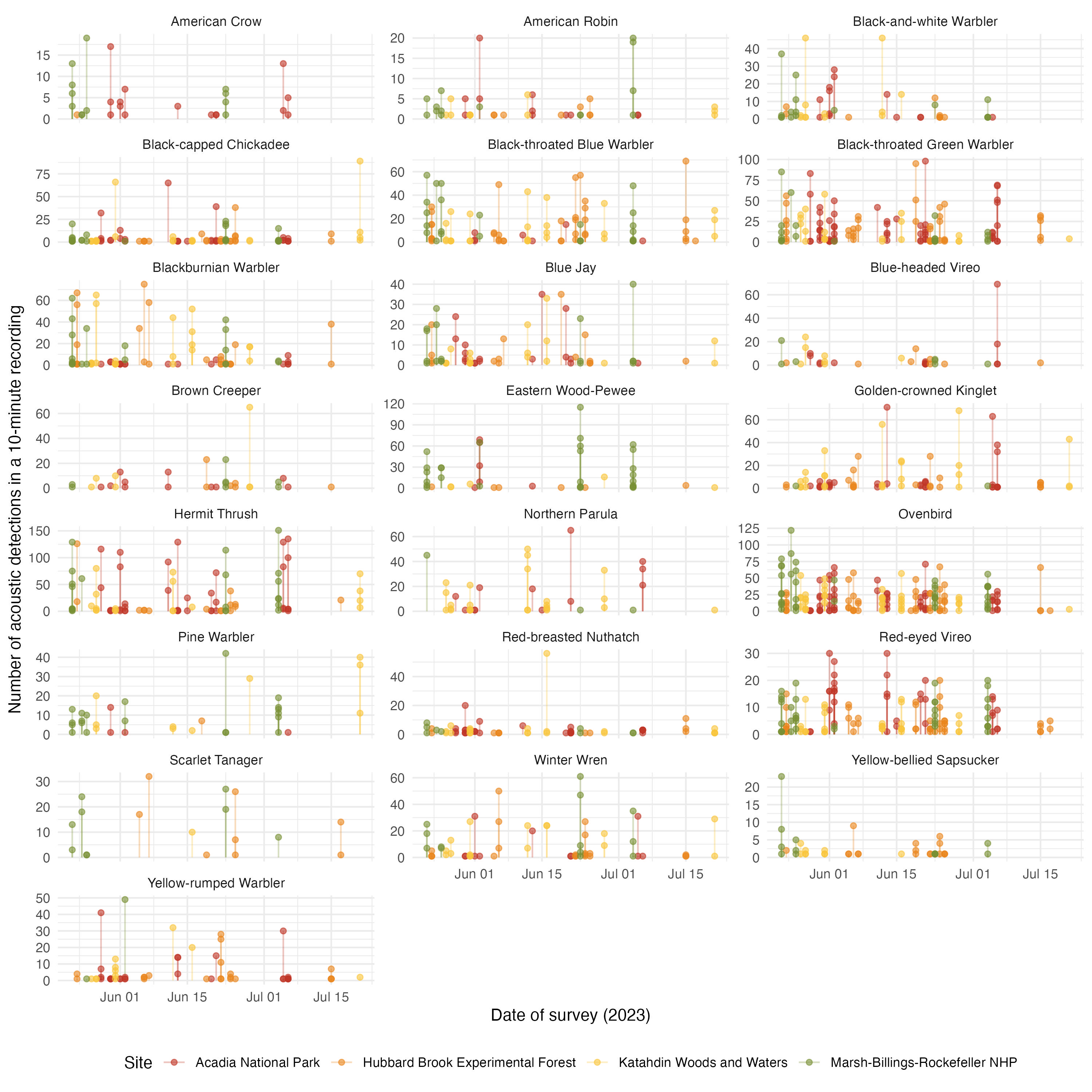
These figures serve to see that the date of visit have a more clear effect in acoustic detections than on counts. We can incorporate these covariates in a hierarchical model.
These figures also allow to estimate the variance-to-mean ratio (VMR) of our two data sources (counts and acoustic detections) to select a family distribution accordingly. Recall a simple, clear table of VMR values:
VMR_table <- data.frame(
  Distribution = c("Constant random variable", "Binomial","Poisson", "Negative binomial"),
  VMR = c("VMR = 0", "0<VMR<1", "VMR = 1", "VMR>1")
)
knitr::kable(VMR_table)
So, estimating these VMR per species:
acoust_count_summary |>
  group_by(common_name) |>
  summarise(meanCounts = mean(counts),
            varCounts = var(counts),
            VMR_counts = varCounts/meanCounts,
            meanAcouDet = mean(acous_detections),
            varAcouDet = var(acous_detections),
            VMR_AcouDet = varAcouDet/meanAcouDet) |> #summary()
  as.data.frame() # to see all the table
We can see that VMR_counts is between 0 and 1, while VMR_AcousticDetection > 1. These ranges suggest using a Binomial and a Negative binomial distributions, respectively, in the observation process.
7.3 Hierarchical model for counts with two observation processes
7.3.1 State process for morning expected counts
Assuming that every morning of sampling we find a latent number of individuals in each site (including several point counts) that fluctuates around a mean stationary number, we can see some similarities with a Stochastic Gompertz State Space population dynamics model, which in continuous time follows a Gaussian (Ornstein-Uhlenbeck, OU) diffusion dynamic.
Let’s model the latent process of log-counts \(X_{i,t} = \ln(C_{i,t})\) for species \(i\) in time \(t\) (sampling point count) in a site \(m\). We can simplify this (for now) by only working in a site (\(m = 1\); Marsh-Billings-Rockefeller NHP) and a single species example (\(i = 1\); Ovenbird - OVEN). On the logarithmic scale, the process becomes linear and follows an autoregressive model of order 1 (note we are not including the index \(m\) nor \(i\) for now):
\[ X_{t+1} = a + c * X_{t} + \epsilon_{t}; ~ \epsilon \sim \text{Normal}(0,\sigma^2) \] where \(a\) control the drift (equivalent to the initial condition at \(t=1\), and then the maximum growth rate in a population model), \(c\) controls the mean-reverting dynamic (such as the strength of density dependence, \(c = 1 + b\) in a population model), and \(\epsilon_{t}\) captures stochasticity in the process, distributed as a normal random variable with some noise of the process \(\sigma^2\). In the long-run, we can estimate the mean of the log-counts as a function of the control drift and mean-reverting dynamic:
\[ \text{E}[X_{\infty}] = \frac{a}{1-c} \]
Also the variance of the log-counts is given by the ratio of variance in stochasticity and the square of the mean-reverting dynamic:
\[ \text{Var}[X_{\infty}] = \frac{\sigma^2}{1-c^2} \]
However, how to deal with Jansen’s inequality?!
\[ e^{(\text{E}[X_\infty])} \leq \text{E}[e^{(X_\infty)}] \]
We can estimate the long-run mean count value on the original scale by adding half of the variance, which is our expected counts per species \(i\):
\[ \text{E}[C_{\infty}] = e^{(\text{E}[X_{\infty}] + (0.5 \times \text{Var}[X_{\infty}]))} \]
7.3.2 Observation process for morning point counts
The VMR_counts revealed underdispersion, so we can us a Binomial distribution for this observation process:
\[ Y_{t}^{Counts} | C_{t} \sim \text{Binomial}(\lambda_{t},~\tau), ~ \lambda_{t} = e^{X_{t}} = C_{t} \] where \(Y_{t}^{counts}\) is the observed counts from point counts sampling, linked to the latent (unobserved) counts \(C_{t}\), assuming that counts are noisy realizations of the true abundance under a binomial distribution with expected “success” counts of \(\lambda_{t}\) and detection probability \(\tau\).
7.3.3 Observation process for morning acoustic detections
The VMR_AcousticDetection revealed overdispersion, so we can use a Negative Binomial distribution for this observation process:
\[ Y_{t}^{AcoustDet}|C_t \sim \text{Negative Binomial}(p_{t}, r) \] where \(Y_{t}^{AcoustDet}\) is the observed acoustic detections from sampling point (that overlap with point counts), \(p_{t} = \frac{r}{r+\lambda_t}\) represents the success parameter, being a ratio of the (over)dispersion parameter \(r\) and the sum of the overdispersion parameter and the mean expected counts \(\lambda_t = e^{X_t} = C_t\). Given that the number of acoustic detection counts does not have a perfect 1:1 relationship with expected counts, we can formulate a log-linear relationship for \(\lambda_t\):
\[ \log(\lambda_{t}) = \alpha + \gamma X_{t} \] where \(\alpha\) is a species-level intercept and \(\gamma\) is the scaling parameter with the latent log-abundance \(X_{t}\).
7.3.4 Coding Observation point counts
Preparing data for data cloning
acoust_count_df <- acoust_count_summary |>
  mutate(Time_w_alone = format(as.POSIXct(Time_window, format = "%Y-%m-%d %H:%M:%S"), "%H:%M"),
         counts = counts+1,
         acous_detections = acous_detections+1,
         year = year(date),
         ) |>
  filter(year == 2022) |>
  arrange(Time_window)

# generate sequence of potential point counts
seq_df <- acoust_count_df |>
  distinct(date) |>   # keep only unique sampled dates
  mutate(seq = map(date, ~ seq(
    from = as.POSIXct(paste(.x, "05:00:00")),
    to   = as.POSIXct(paste(.x, "10:00:00")),
    by   = "10 min"
  ))) |>
  unnest(seq) |>
  mutate(Time_window = seq,
         Time_w_alone = format(seq, "%H:%M"))

final_df <- seq_df |>
  select(c(date, Time_w_alone)) |>
  left_join(acoust_count_df, by = c("date", "Time_w_alone"))

final_df$DateTime <- as.POSIXct(paste(final_df$date, final_df$Time_w_alone), format = "%Y-%m-%d %H:%M")

final_df$time_id <- as.integer(factor(final_df$DateTime))
StochGSS.dc <- function(){
# Priors on model parameters. Priors are DC1 in Lele et al (2007)
a1 ~ dnorm(0,1); # constant, equivalent to the population growth rate.
c1 ~ dunif(-1,1); # constant, the density dependence parameter.
sig1 ~ dlnorm(-0.5,10); #variance parameter of stochastic environment (process noise) in the system
stovar1 <- 1/pow(sig1,2)
tau1 ~ dunif(0,1); # detection probability in Binomial distribution
for(k in 1:K){
# Simulate trajectory that depends on the previous
mean_X1[1,k] <- a1/(1-c1) # Expected value of the first realization of the process
# this is drawn from the stationary distribution of the process
# Equation 14 (main text) and A.4 in Appendix of Dennis et al 2006
Varno1[k] <- pow(sig1,2)/(1-pow(c1,2)) #. Equation A.5 in Appendix of Dennis et al 2006
# Updating the state: Stochastic process for all time steps
X1[1,k]~dnorm(mean_X1[1,k], 1/Varno1[k]); #first estimation of population
#iteration of the GSS model in the data
for (t in 2:qp1) {
mean_X1[t,k] <- a1 + c1 * X1[(t - 1),k]
X1[t,k] ~ dnorm(mean_X1[t,k], stovar1) # Et is included here since a+cX(t-1) + Et ~ Normal(a+cX(t-1),sigma^2)
}
# Updating the observations, from the counts under Binomial observation error
for (t in 1:qp1) {
N1[t,k] ~ dpois(exp(X1[t,k])) # trick to convert continuous exp(X1) to integer counts as trials
Y1[t,k] ~ dbin(tau1, N1[t,k]) #
}
}
}For this model, we will need some initial values of the parameters, and given that there could be many NA a wrap to provide those initial guess values.
guess.calc <- function(Yobs,Tvec){

  T.t <-Tvec-Tvec[1]; #  For calculations, time starts at zero.
  q <- length(Yobs)-1;      #  Number of time series transitions, q.
  qp1 <- q+1;              #  q+1 gets used a lot, too.
  S.t <- T.t[2:qp1]-T.t[1:q];  #  Time intervals.
  Ybar <- mean(Yobs);
  Yvar <- sum((Yobs-Ybar)*(Yobs-Ybar))/q;
  mu1 <- Ybar;

  # Kludge an initial value for theta based on mean of Y(t+s) given Y(t).
  th1<- -mean(log(abs((Yobs[2:qp1]-mu1)/(Yobs[1:q]-mu1)))/S.t);
  bsq1<- 2*th1*Yvar/(1+2*th1);         # Moment estimate using stationary
  tsq1<- bsq1;                         #   variance, with betasq=tausq.

  #three 0's
  three0s <- sum(c(th1,bsq1,tsq1))
  if(three0s==0|is.na(three0s)){th1 <- 0.5;bsq1 <- 0.09; tsq1 <- 0.23;}


  out1 <- c(th1,bsq1,tsq1);
  if(sum(out1<1e-7)>=1){out1 <- c(0.5,0.09,0.23)}
  out <- c(mu1,out1);
  return(abs(out))

}

guess.calc2.0<- function(TimeAndNs){

  newmat <- TimeAndNs
  isnas <- sum(is.na(TimeAndNs))

  if(isnas >= 1){

    isnaind <- which(is.na(TimeAndNs[,2]), arr.ind=TRUE)
    newmat <- TimeAndNs[-isnaind,]
    newmat[,1] <- newmat[,1] - newmat[1,1]

  }

  init.guess <- guess.calc(Yobs = log(newmat[,2]), Tvec=newmat[,1])

  mu1  <- init.guess[1]
  th1  <- init.guess[2]
  bsq1 <- init.guess[3]
  sigsq1<- ((1-exp(-2*th1))*bsq1)/(2*th1)

  out <- c(mu=mu1, theta=th1, sigmasq = sigsq1)
  return(out)
}
And we have to bundle the data for Data cloning. Let’s fit the first species in the taxa with higher data (Ovenbird in Marsh-Billings-Rockefeller NHP) as a test.
ts.4guess  <-  final_df$counts
tvec4guess  <- 1:length(ts.4guess)
onets4guess <- cbind(tvec4guess, ts.4guess)
naive.guess <- guess.calc2.0(TimeAndNs = onets4guess)

datalistGSS.dc <- list(K = 1,
                       qp1 = length(ts.4guess),
                       Y1 = dcdim(array(ts.4guess,
                                        dim = c(length(ts.4guess),1))))

dcrun.GSS <- dc.fit(data = datalistGSS.dc,
                    params = c("a1", "c1", "sig1", "tau1"),
                    model = StochGSS.dc,
                    n.clones = c(1,5,10,20),
                    multiply = "K",
                    unchanged = "qp1",
                    n.chains = 3,
                    n.adapt = 5000,
                    n.update = 100,
                    thin = 20,
                    n.iter = 20000)

saveRDS(dcrun.GSS, "data/dcfitGSS_2022_OVEN_MBR.rds")
dcrun.GSS <- readRDS("data/dcfitGSS_2022_OVEN_MBR.rds")
summary(dcrun.GSS);
dcdiag(dcrun.GSS)
plot(dcdiag(dcrun.GSS))
pairs(dcrun.GSS)
coef(dcrun.GSS)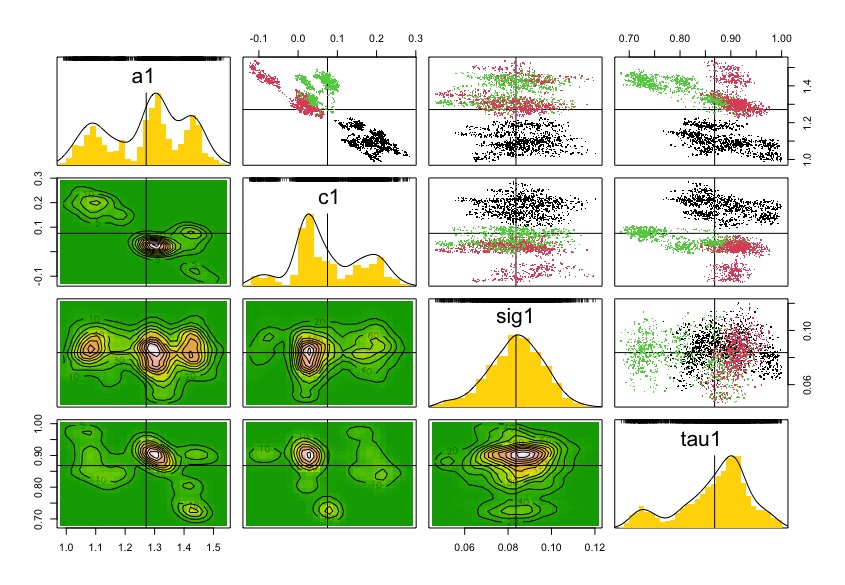
And with these coefficients of the model, we can estimate latent count trajectories with the Kalman filter structure. This Kalman filter structure allows simultaneous estimation of latent states for observed time steps and prediction for missing ones, leveraging the temporal correlation in the process model.
Kalman.pred.fn <- function() {
# Priors on model parameters: they are on the real line.
  parms ~ dmnorm(MuPost,PrecPost)
  a1 <- parms[1]
  c1 <- parms[2]
  sig1 <- parms[3]
  stovar1 <- 1/pow(sig1,2)
  tau1 ~ dunif(0,1)

  # Likelihood
  mean_X1[1] <- a1/(1-c1) # Expected value of the first realization of the process
    # this is drawn from the stationary distribution of the process
    # Equation 14 (main text) and  A.4 in Appendix of Dennis et al 2006
    Varno1 <- pow(sig1,2)/(1-pow(c1,2)) #. Equation A.5 in Appendix of Dennis et al 2006

    # Updating the state: Stochastic process for all time steps
    X1[1]~dnorm(mean_X1[1], 1/Varno1); #first estimation of population
    C[1] <- exp(X1[1])
    #iteration of the GSS model in the data
    for (t in 2:qp1) {
      mean_X1[t] <- a1 + c1 * X1[(t - 1)]
      X1[t] ~ dnorm(mean_X1[t], stovar1) # Et is included here since a+cX(t-1) + Et ~ Normal(a+cX(t-1),sigma^2)
      N[t] ~ dpois(exp(X1[t]))   # trick to convert continuous exp(X1) to integer counts as trials in binomial
      Y1[(t-1)] ~ dbin(tau1, N[t])   #
      C[t] <- exp(X1[t]) # expected count
    }
}
data4kalman <- list(qp1 = as.numeric(length(final_df$counts)),
Y1 = array(final_df$counts,
dim = c(as.numeric(length(final_df$counts)))),
MuPost = coef(dcrun.GSS),
PrecPost = solve(vcov(dcrun.GSS))) And run the Bayesian inference using the MLE from Data cloning
And we can generate a dataframe of the time series with the estimates, inter quartile range, and observed data through time
summary(BH_DC_Pred)
# extract predictions and CI around them
pred <- as.data.frame(t(mcmcapply(BH_DC_Pred, quantile, c(0.025, 0.5, 0.975))))

ExpectedCounts <- as.data.frame(cbind(final_df,pred))
# modify names
names(ExpectedCounts) <- c("date","Time_w_alone","site_name","site_id",
                          "visit_number","common_name","time_window",
                          "Observed",
                          "acous_detections","DateTime","Time_window", "year",
                          "time_id","Lower", "Estimated", "Upper")


ExpectedCounts |>
  pivot_longer(cols = c(Lower, Estimated, Upper, Observed),
               names_to = "Abundance",
               values_to = "Count") |>
  ggplot(aes(x = DateTime,
             y = Count,
             color = factor(Abundance,
                            levels = c("Observed",
                                       "Upper",
                                       "Estimated",
                                       "Lower")))) +
    geom_line(aes(linetype = factor(Abundance,
                            levels = c("Observed",
                                       "Upper",
                                       "Estimated",
                                       "Lower")))) +
    geom_point(aes(shape = factor(Abundance,
                            levels = c("Observed",
                                       "Upper",
                                       "Estimated",
                                       "Lower")))) +
    labs(title = "OVEN - Marsh-Billings-Rockefeller NHP - 2022 sampling",
         x = "Time (sampling window)",
         y = "Counts",
         color = "Counts",
         linetype = "Counts",
         shape = "Counts") +
    scale_linetype_manual(values = c(NA,"dashed","solid","dashed"))+
    scale_shape_manual(values = c(21, NA,NA,NA)) +
    scale_color_manual(values = c("blue","darkgray","black","darkgray")) +
    theme_classic() +
    theme(legend.position = "bottom")
7.3.5 Coding Acoustic detections counts
StochGSS.acou.dc <- function(){

  # Priors on model parameters. Priors are DC1 in Lele et al (2007)
  a1 ~ dnorm(0,1);        # constant, equivalent to the population growth rate.
  c1 ~ dunif(-1,1);       # constant, the density dependence parameter.
  sig1 ~ dlnorm(-0.5,10); #variance parameter of stochastic  environment (process noise) in the system
  stovar1 <- 1/pow(sig1,2)

   # Priors for observation model
  alpha ~ dnorm(0, 0.001)  # intercept for scaling
  gamma ~ dnorm(0, 0.001)  # slope linking latent state X_t to mean
  r ~ dunif(0,50)   # dispersion parameter for NegBin

  for(k in 1:K){
    # Simulate trajectory that depends on the previous
    mean_X1[1,k] <- a1/(1-c1) # Expected value of the first realization of the process
    # this is drawn from the stationary distribution of the process
    # Equation 14 (main text) and  A.4 in Appendix of Dennis et al 2006
    Varno1[k] <- pow(sig1,2)/(1-pow(c1,2)) #. Equation A.5 in Appendix of Dennis et al 2006

    # Updating the state: Stochastic process for all time steps
    X1[1,k]~dnorm(mean_X1[1,k], 1/Varno1[k]); #first estimation of population

    #iteration of the GSS model in the data
    for (t in 2:qp1) {
      mean_X1[t,k] <- a1 + c1 * X1[(t - 1),k]
      X1[t,k] ~ dnorm(mean_X1[t,k], stovar1) # Et is included here since a+cX(t-1) + Et ~ Normal(a+cX(t-1),sigma^2)
    }

    # Updating the observations, from the acoustic detections under Negative Binomial observation error
    for (t in 1:qp1) {
      Y1[t,k] ~ dnegbin(p[t,k], r)
      p[t,k] <- r/(r+lambda[t,k])
      log(lambda[t,k]) <- alpha + gamma * X1[t,k]
      }
  }
}
For this model, we will need some initial values of the parameters, and given that there could be many NA a wrap to provide those initial guess values.
guess.calc <- function(Yobs,Tvec){

  T.t <-Tvec-Tvec[1]; #  For calculations, time starts at zero.
  q <- length(Yobs)-1;      #  Number of time series transitions, q.
  qp1 <- q+1;              #  q+1 gets used a lot, too.
  S.t <- T.t[2:qp1]-T.t[1:q];  #  Time intervals.
  Ybar <- mean(Yobs);
  Yvar <- sum((Yobs-Ybar)*(Yobs-Ybar))/q;
  mu1 <- Ybar;

  # Kludge an initial value for theta based on mean of Y(t+s) given Y(t).
  th1<- -mean(log(abs((Yobs[2:qp1]-mu1)/(Yobs[1:q]-mu1)))/S.t);
  bsq1<- 2*th1*Yvar/(1+2*th1);         # Moment estimate using stationary
  tsq1<- bsq1;                         #   variance, with betasq=tausq.

  #three 0's
  three0s <- sum(c(th1,bsq1,tsq1))
  if(three0s==0|is.na(three0s)){th1 <- 0.5;bsq1 <- 0.09; tsq1 <- 0.23;}


  out1 <- c(th1,bsq1,tsq1);
  if(sum(out1<1e-7)>=1){out1 <- c(0.5,0.09,0.23)}
  out <- c(mu1,out1);
  return(abs(out))

}

guess.calc2.0<- function(TimeAndNs){

  newmat <- TimeAndNs
  isnas <- sum(is.na(TimeAndNs))

  if(isnas >= 1){

    isnaind <- which(is.na(TimeAndNs[,2]), arr.ind=TRUE)
    newmat <- TimeAndNs[-isnaind,]
    newmat[,1] <- newmat[,1] - newmat[1,1]

  }

  init.guess <- guess.calc(Yobs = log(newmat[,2]), Tvec=newmat[,1])

  mu1  <- init.guess[1]
  th1  <- init.guess[2]
  bsq1 <- init.guess[3]
  sigsq1<- ((1-exp(-2*th1))*bsq1)/(2*th1)

  out <- c(mu=mu1, theta=th1, sigmasq = sigsq1)
  return(out)
}
And we have to bundle the data for Data cloning. Let’s fit the first species in the taxa with higher data (Ovenbird in Marsh-Billings-Rockefeller NHP) as a test.
ts.4guess  <-  as.numeric(final_df$acous_detections)
tvec4guess  <- 1:length(ts.4guess)
onets4guess <- cbind(tvec4guess, ts.4guess)
naive.guess <- guess.calc2.0(TimeAndNs = onets4guess)

datalistGSS.acou.dc <- list(K = 1,
                       qp1 = length(ts.4guess),
                       Y1 = dcdim(array(ts.4guess,
                                        dim = c(length(ts.4guess),1))))

dcrun.GSS.acou <- dc.fit(data = datalistGSS.acou.dc,
                    params = c("a1", "c1", "sig1", "gamma", "alpha", "r"),
                    model = StochGSS.acou.dc,
                    n.clones = c(1,5,10,20),
                    multiply = "K",
                    unchanged = "qp1",
                    n.chains = 3,
                    n.adapt = 5000,
                    n.update = 100,
                    thin = 20,
                    n.iter = 20000)

saveRDS(dcrun.GSS.acou, "data/dcfitGSS_AcDet_2022_OVEN_MBR.rds")
dcrun.GSS.acou <- readRDS("data/dcfitGSS_AcDet_2022_OVEN_MBR.rds")
summary(dcrun.GSS.acou);
dcdiag(dcrun.GSS.acou)
plot(dcdiag(dcrun.GSS.acou))
pairs(dcrun.GSS.acou)
coef(dcrun.GSS.acou)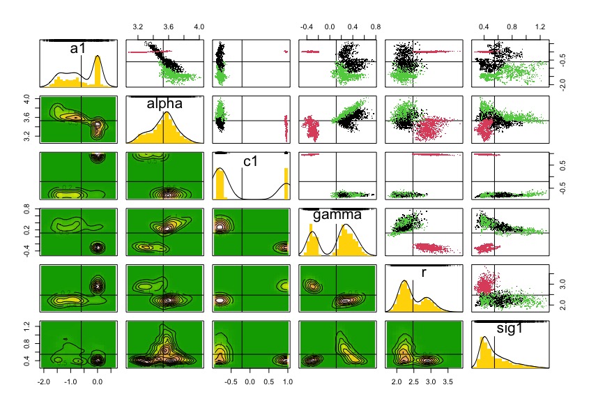
Although diagnostics for lambda.max decreases with more clones, the chains are not converging. It seems that this needs more iterations and change initial values.
Anyway, with these coefficients of the model, we can estimate latent count trajectories with the Kalman filter structure. This Kalman filter structure allows simultaneous estimation of latent states for observed time steps and prediction for missing ones, leveraging the temporal correlation in the process model.
Kalman.pred.acou.fn <- function() {
# Priors on model parameters: they are on the real line.
  parms ~ dmnorm(MuPost,PrecPost)
  a1 <- parms[1]
  alpha <- parms[2]   # intercept for scaling
  c1 <- parms[3]
  gamma <- parms[4]  # slope linking latent state X_t to mean
  r <- parms[5]      # overdispersion parameter for NegBinom
  sig1 <- parms[6]
  stovar1 <- 1/pow(sig1,2)

  # Likelihood
  mean_X1[1] <- a1/(1-c1) # Expected value of the first realization of the process
    # this is drawn from the stationary distribution of the process
    # Equation 14 (main text) and  A.4 in Appendix of Dennis et al 2006
    Varno1 <- pow(sig1,2)/(1-pow(c1,2)) #. Equation A.5 in Appendix of Dennis et al 2006

    # Updating the state: Stochastic process for all time steps
    X1[1]~dnorm(mean_X1[1], 1/Varno1); #first estimation of population
    log(lambda[1]) <- alpha + gamma * X1[1]
    C[1] <- log(lambda[1])
    #iteration of the GSS model in the data
    for (t in 2:qp1) {
      mean_X1[t] <- a1 + c1 * X1[(t - 1)]
      X1[t] ~ dnorm(mean_X1[t], stovar1) # Et is included here since a+cX(t-1) + Et ~ Normal(a+cX(t-1),sigma^2)

      Y1[(t-1)] ~ dnegbin(p[t], r)
      p[t] <- r/(r+lambda[t])
      log(lambda[t]) <- alpha + gamma * X1[t]
      C[t] <- log(lambda[t]) # expected count
    }
}
data4kalmanAco <- list(qp1 = as.numeric(length(final_df$acous_detections)),
Y1 = array(final_df$acous_detections,
dim = c(as.numeric(length(final_df$acous_detections)))),
MuPost = coef(dcrun.GSS.acou),
PrecPost = solve(vcov(dcrun.GSS.acou))) And run the Bayesian inference using the MLE from Data cloning
And we can generate a dataframe of the time series with the estimates, inter quartile range, and observed data through time
summary(BH_DC_Pred_Acou)
# extract predictions and CI around them
predAcou <- as.data.frame(t(mcmcapply(BH_DC_Pred_Acou, quantile, c(0.025, 0.5, 0.975))))


ExpectedCountsAcou <- as.data.frame(cbind(ExpectedCounts,predAcou))
# modify names
names(ExpectedCountsAcou) <- c("date","Time_w_alone","site_name","site_id",
                          "visit_number","common_name","time_window",
                          "Observed",
                          "AcousticDetections",
                          "DateTime","Time_window", "year",
                          "time_id",
                          "CountLower", "CountEstimated", "CountUpper",
                          "AcouDetLower", "AcouDetEstimated", "AcouDetUpper")

par(mar = c(5, 4, 7, 2))  # low, left, up, right

plot(x = ExpectedCountsAcou$DateTime,
     y = ExpectedCountsAcou$Observed,
     col = "#1b7837",
     ylim = c(0,40),
     ylab = "Counts",
     xlab = "Time (sampling window)")
points(x = ExpectedCountsAcou$DateTime,
     y = ExpectedCountsAcou$AcousticDetections,
     col = "#762a83")
lines(x = ExpectedCountsAcou$DateTime,
     y = ExpectedCountsAcou$CountEstimated,
     col = "#7fbf7b")
lines(x = ExpectedCountsAcou$DateTime,
     y = ExpectedCountsAcou$CountLower,
     col = "#d9f0d3", lty = 2)
lines(x = ExpectedCountsAcou$DateTime,
     y = ExpectedCountsAcou$CountUpper,
     col = "#d9f0d3", lty = 2)
lines(x = ExpectedCountsAcou$DateTime,
     y = ExpectedCountsAcou$AcouDetEstimated,
     col = "#af8dc3")
lines(x = ExpectedCountsAcou$DateTime,
     y = ExpectedCountsAcou$AcouDetLower,
     col = "#e7d4e8", lty = 2)
lines(x = ExpectedCountsAcou$DateTime,
     y = ExpectedCountsAcou$AcouDetUpper,
     col = "#e7d4e8", lty = 2)

legend(x = min(ExpectedCountsAcou$DateTime),
       y = 65,
       cex = 0.7,
       pt.cex = 0.7,
       xpd = TRUE,
       horiz = FALSE,
       legend = c("Observed from point counts",
                  "Acoustic detections",
                  "Estimate from point counts",
                  "Point count CI estimates",
                  "Estimate from acoustic detections",
                  "Acoustic detections CI estimates"),
       col = c("#1b7837",
               "#762a83",
               "#7fbf7b",
               "#d9f0d3",
               "#af8dc3",
               "#e7d4e8"),
       lty = c(NA, NA, 1, 2, 1, 2),   # NA for points, 1 for solid lines, 2 for dashed
       pch = c(1, 1, NA, NA, NA, NA), # symbols for points
       bty = "n")                     # no box around legend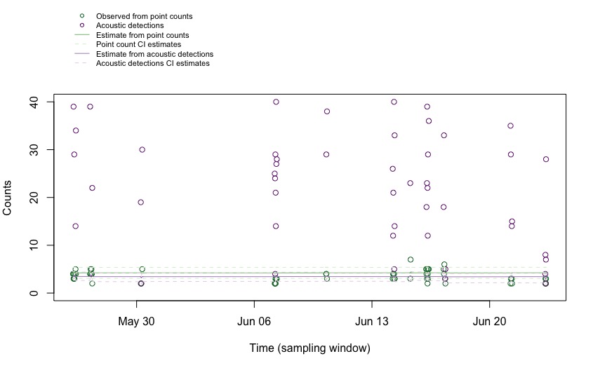
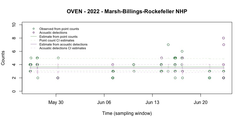
Cutting the edges to see the details of the estimates:
par(mar = c(6, 4, 4, 2))

plot(x = ExpectedCountsAcou$DateTime,
     y = ExpectedCountsAcou$Observed,
     col = "#1b7837",
     ylim = c(0,10),
     ylab = "Counts",
     xlab = "Time (sampling window)",
     main = "OVEN - 2022 - Marsh-Billings-Rockefeller NHP")
points(x = ExpectedCountsAcou$DateTime,
     y = ExpectedCountsAcou$AcousticDetections,
     col = "#762a83")
lines(x = ExpectedCountsAcou$DateTime,
     y = ExpectedCountsAcou$CountEstimated,
     col = "#7fbf7b")
lines(x = ExpectedCountsAcou$DateTime,
     y = ExpectedCountsAcou$CountLower,
     col = "#d9f0d3", lty = 2)
lines(x = ExpectedCountsAcou$DateTime,
     y = ExpectedCountsAcou$CountUpper,
     col = "#d9f0d3", lty = 2)
lines(x = ExpectedCountsAcou$DateTime,
     y = ExpectedCountsAcou$AcouDetEstimated,
     col = "#af8dc3")
lines(x = ExpectedCountsAcou$DateTime,
     y = ExpectedCountsAcou$AcouDetLower,
     col = "#e7d4e8", lty = 2)
lines(x = ExpectedCountsAcou$DateTime,
     y = ExpectedCountsAcou$AcouDetUpper,
     col = "#e7d4e8", lty = 2)

legend(x = min(ExpectedCountsAcou$DateTime),
       y = 10,
       cex = 0.7,
       pt.cex = 0.7,
       xpd = TRUE,
       horiz = FALSE,
       legend = c("Observed from point counts",
                  "Acoustic detections",
                  "Estimate from point counts",
                  "Point count CI estimates",
                  "Estimate from acoustic detections",
                  "Acoustic detections CI estimates"),
       col = c("#1b7837",
               "#762a83",
               "#7fbf7b",
               "#d9f0d3",
               "#af8dc3",
               "#e7d4e8"),
       lty = c(NA, NA, 1, 2, 1, 2),   # NA for points, 1 for solid lines, 2 for dashed
       pch = c(1, 1, NA, NA, NA, NA), # symbols for points
       bty = "n")                     # no box around legend