Section 8 Another example with hierarchical model approach - OVEN in Katahdin Woods and Waters
8.2 Loading and exploring data
Let’s load the file used in 01_data-comparability.Rmd script.
Let’s work on the species-site combination of more data: Ovenbird in Marsh-Billings-Rockefeller NHP.
acous_count_filt <- acous_count |>
  filter(common_name %in% c(
    #"American Crow","American Robin","Black-and-white Warbler","Black-capped Chickadee","Black-throated Blue Warbler","Black-throated Green Warbler","Blackburnian Warbler","Blue Jay","Blue-headed Vireo","Brown Creeper","Eastern Wood-Pewee","Golden-crowned Kinglet","Hermit Thrush","Northern Parula",

                            "Ovenbird"

                            #,"Pine Warbler","Red-breasted Nuthatch","Red-eyed Vireo","Scarlet Tanager","Winter Wren","Yellow-bellied Sapsucker","Yellow-rumped Warbler"
                            ),
    site_name == "Katahdin Woods and Waters")
table(acous_count_filt$common_name, acous_count_filt$data_type)
How to reconcile time of detection of each record?
While the point_count data include the observation_time variable, this information for the acoustic_data seems to be at the begin_clock_time variable. Let’s adjust this with the function coalesce from dplyr in tidyverse. Then, we can consolidate the “initial temporal window” per visit in each site_id with the detection time.
acoust_count_summary <- acous_count_filt |>
  # dummy column to unify time of detection either by count or
  mutate(detection_time = coalesce(observation_time, begin_clock_time)) |>
  # initial temporal window
  group_by(site_id, date, visit_number) |>
  mutate(time_window = min(hms::as_hms(detection_time), na.rm = TRUE),
         time_window = hms::as_hms(time_window)) |>
  # First summarization to extract sum of counts per point count and number of detections
  group_by(site_name, site_id, date, visit_number, common_name, data_type, time_window, detection_time) |>
  summarise(abundance = sum(abundance, na.rm = TRUE),
         acous_detections = n()) |>
  # Second summarization to count number of detections and extract overall counts
  group_by(site_name, site_id, date, visit_number, common_name, time_window) |>
  summarise(counts = sum(abundance, na.rm = TRUE),
         acous_detections = sum(acous_detections)) |>
  as.data.frame()

acoust_count_summary$DateTime <- as.POSIXct(paste(acoust_count_summary$date, acoust_count_summary$time_window), format = "%Y-%m-%d %H:%M:%S")

acoust_count_summary$Time_window <- floor_date(acoust_count_summary$DateTime, "10 mins")

str(acoust_count_summary)
And we can generate the figures. This are similar to my previous attempt, but including some days or point counts discarded by Vijay due to species richness.
8.3 Hierarchical model for counts with two observation processes
8.3.1 Coding Observation point counts
Preparing data for data cloning
acoust_count_df <- acoust_count_summary |>
  mutate(Time_w_alone = format(as.POSIXct(Time_window, format = "%Y-%m-%d %H:%M:%S"), "%H:%M"),
         counts = counts+1,
         acous_detections = acous_detections+1,
         year = year(date),
         ) |>
  filter(year == 2023) |>
  arrange(Time_window)

# generate sequence of potential point counts
seq_df <- acoust_count_df |>
  distinct(date) |>   # keep only unique sampled dates
  mutate(seq = map(date, ~ seq(
    from = as.POSIXct(paste(.x, "05:00:00")),
    to   = as.POSIXct(paste(.x, "10:00:00")),
    by   = "10 min"
  ))) |>
  unnest(seq) |>
  mutate(Time_window = seq,
         Time_w_alone = format(seq, "%H:%M"))

final_df <- seq_df |>
  select(c(date, Time_w_alone)) |>
  left_join(acoust_count_df, by = c("date", "Time_w_alone"))

final_df$DateTime <- as.POSIXct(paste(final_df$date, final_df$Time_w_alone), format = "%Y-%m-%d %H:%M")

final_df$time_id <- as.integer(factor(final_df$DateTime))
StochGSS.dc <- function(){
# Priors on model parameters. Priors are DC1 in Lele et al (2007)
a1 ~ dnorm(0,1); # constant, equivalent to the population growth rate.
c1 ~ dunif(-1,1); # constant, the density dependence parameter.
sig1 ~ dlnorm(-0.5,10); #variance parameter of stochastic environment (process noise) in the system
stovar1 <- 1/pow(sig1,2)
tau1 ~ dunif(0,1); # detection probability in Binomial distribution
for(k in 1:K){
# Simulate trajectory that depends on the previous
mean_X1[1,k] <- a1/(1-c1) # Expected value of the first realization of the process
# this is drawn from the stationary distribution of the process
# Equation 14 (main text) and A.4 in Appendix of Dennis et al 2006
Varno1[k] <- pow(sig1,2)/(1-pow(c1,2)) #. Equation A.5 in Appendix of Dennis et al 2006
# Updating the state: Stochastic process for all time steps
X1[1,k]~dnorm(mean_X1[1,k], 1/Varno1[k]); #first estimation of population
#iteration of the GSS model in the data
for (t in 2:qp1) {
mean_X1[t,k] <- a1 + c1 * X1[(t - 1),k]
X1[t,k] ~ dnorm(mean_X1[t,k], stovar1) # Et is included here since a+cX(t-1) + Et ~ Normal(a+cX(t-1),sigma^2)
}
# Updating the observations, from the counts under Binomial observation error
for (t in 1:qp1) {
N1[t,k] ~ dpois(exp(X1[t,k])) # trick to convert continuous exp(X1) to integer counts as trials
Y1[t,k] ~ dbin(tau1, N1[t,k]) #
}
}
}For this model, we will need some initial values of the parameters, and given that there could be many NA a wrap to provide those initial guess values.
guess.calc <- function(Yobs,Tvec){

  T.t <-Tvec-Tvec[1]; #  For calculations, time starts at zero.
  q <- length(Yobs)-1;      #  Number of time series transitions, q.
  qp1 <- q+1;              #  q+1 gets used a lot, too.
  S.t <- T.t[2:qp1]-T.t[1:q];  #  Time intervals.
  Ybar <- mean(Yobs);
  Yvar <- sum((Yobs-Ybar)*(Yobs-Ybar))/q;
  mu1 <- Ybar;

  # Kludge an initial value for theta based on mean of Y(t+s) given Y(t).
  th1<- -mean(log(abs((Yobs[2:qp1]-mu1)/(Yobs[1:q]-mu1)))/S.t);
  bsq1<- 2*th1*Yvar/(1+2*th1);         # Moment estimate using stationary
  tsq1<- bsq1;                         #   variance, with betasq=tausq.

  #three 0's
  three0s <- sum(c(th1,bsq1,tsq1))
  if(three0s==0|is.na(three0s)){th1 <- 0.5;bsq1 <- 0.09; tsq1 <- 0.23;}


  out1 <- c(th1,bsq1,tsq1);
  if(sum(out1<1e-7)>=1){out1 <- c(0.5,0.09,0.23)}
  out <- c(mu1,out1);
  return(abs(out))

}

guess.calc2.0<- function(TimeAndNs){

  newmat <- TimeAndNs
  isnas <- sum(is.na(TimeAndNs))

  if(isnas >= 1){

    isnaind <- which(is.na(TimeAndNs[,2]), arr.ind=TRUE)
    newmat <- TimeAndNs[-isnaind,]
    newmat[,1] <- newmat[,1] - newmat[1,1]

  }

  init.guess <- guess.calc(Yobs = log(newmat[,2]), Tvec=newmat[,1])

  mu1  <- init.guess[1]
  th1  <- init.guess[2]
  bsq1 <- init.guess[3]
  sigsq1<- ((1-exp(-2*th1))*bsq1)/(2*th1)

  out <- c(mu=mu1, theta=th1, sigmasq = sigsq1)
  return(out)
}
And we have to bundle the data for Data cloning. Let’s fit the first species in the taxa with higher data (Ovenbird in Marsh-Billings-Rockefeller NHP) as a test.
ts.4guess  <-  final_df$counts
tvec4guess  <- 1:length(ts.4guess)
onets4guess <- cbind(tvec4guess, ts.4guess)
naive.guess <- guess.calc2.0(TimeAndNs = onets4guess)

datalistGSS.dc <- list(K = 1,
                       qp1 = length(ts.4guess),
                       Y1 = dcdim(array(ts.4guess,
                                        dim = c(length(ts.4guess),1))))

dcrun.GSS <- dc.fit(data = datalistGSS.dc,
                    params = c("a1", "c1", "sig1", "tau1"),
                    model = StochGSS.dc,
                    n.clones = c(1,5,10,20),
                    multiply = "K",
                    unchanged = "qp1",
                    n.chains = 3,
                    n.adapt = 5000,
                    n.update = 100,
                    thin = 20,
                    n.iter = 20000)

saveRDS(dcrun.GSS, "data/dcfitGSS_2023_OVEN_KWW.rds")
dcrun.GSS <- readRDS("data/dcfitGSS_2023_OVEN_KWW.rds")
summary(dcrun.GSS);
dcdiag(dcrun.GSS)
plot(dcdiag(dcrun.GSS))
pairs(dcrun.GSS)
coef(dcrun.GSS)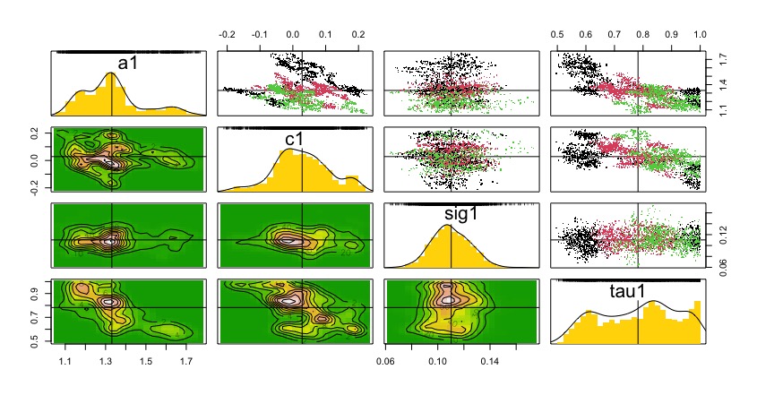
And with these coefficients of the model, we can estimate latent count trajectories with the Kalman filter structure. This Kalman filter structure allows simultaneous estimation of latent states for observed time steps and prediction for missing ones, leveraging the temporal correlation in the process model.
Kalman.pred.fn <- function() {
# Priors on model parameters: they are on the real line.
  parms ~ dmnorm(MuPost,PrecPost)
  a1 <- parms[1]
  c1 <- parms[2]
  sig1 <- parms[3]
  stovar1 <- 1/pow(sig1,2)
  tau1 ~ dunif(0,1)

  # Likelihood
  mean_X1[1] <- a1/(1-c1) # Expected value of the first realization of the process
    # this is drawn from the stationary distribution of the process
    # Equation 14 (main text) and  A.4 in Appendix of Dennis et al 2006
    Varno1 <- pow(sig1,2)/(1-pow(c1,2)) #. Equation A.5 in Appendix of Dennis et al 2006

    # Updating the state: Stochastic process for all time steps
    X1[1]~dnorm(mean_X1[1], 1/Varno1); #first estimation of population
    C[1] <- exp(X1[1])
    #iteration of the GSS model in the data
    for (t in 2:qp1) {
      mean_X1[t] <- a1 + c1 * X1[(t - 1)]
      X1[t] ~ dnorm(mean_X1[t], stovar1) # Et is included here since a+cX(t-1) + Et ~ Normal(a+cX(t-1),sigma^2)
      N[t] ~ dpois(exp(X1[t]))   # trick to convert continuous exp(X1) to integer counts as trials in binomial
      Y1[(t-1)] ~ dbin(tau1, N[t])   #
      C[t] <- exp(X1[t]) # expected count
    }
}
data4kalman <- list(qp1 = as.numeric(length(final_df$counts)),
Y1 = array(final_df$counts,
dim = c(as.numeric(length(final_df$counts)))),
MuPost = coef(dcrun.GSS),
PrecPost = solve(vcov(dcrun.GSS))) And run the Bayesian inference using the MLE from Data cloning
And we can generate a dataframe of the time series with the estimates, inter quartile range, and observed data through time
summary(BH_DC_Pred)
# extract predictions and CI around them
pred <- as.data.frame(t(mcmcapply(BH_DC_Pred, quantile, c(0.025, 0.5, 0.975))))

ExpectedCounts <- as.data.frame(cbind(final_df,pred))
# modify names
names(ExpectedCounts) <- c("date","Time_w_alone","site_name","site_id",
                          "visit_number","common_name","time_window",
                          "Observed",
                          "acous_detections","DateTime","Time_window", "year",
                          "time_id","Lower", "Estimated", "Upper")


ExpectedCounts |>
  pivot_longer(cols = c(Lower, Estimated, Upper, Observed),
               names_to = "Abundance",
               values_to = "Count") |>
  ggplot(aes(x = DateTime,
             y = Count,
             color = factor(Abundance,
                            levels = c("Observed",
                                       "Upper",
                                       "Estimated",
                                       "Lower")))) +
    geom_line(aes(linetype = factor(Abundance,
                            levels = c("Observed",
                                       "Upper",
                                       "Estimated",
                                       "Lower")))) +
    geom_point(aes(shape = factor(Abundance,
                            levels = c("Observed",
                                       "Upper",
                                       "Estimated",
                                       "Lower")))) +
  scale_y_continuous(limits = c(0,10))+
    labs(title = "OVEN - Katahdin Woods and Waters - 2023 sampling",
         x = "Time (sampling window)",
         y = "Counts",
         color = "Counts",
         linetype = "Counts",
         shape = "Counts") +
    scale_linetype_manual(values = c(NA,"dashed","solid","dashed"))+
    scale_shape_manual(values = c(21, NA,NA,NA)) +
    scale_color_manual(values = c("blue","darkgray","black","darkgray")) +
    theme_classic() +
    theme(legend.position = "bottom")
8.3.2 Coding Acoustic detections counts
StochGSS.acou.dc <- function(){

  # Priors on model parameters. Priors are DC1 in Lele et al (2007)
  a1 ~ dnorm(0,1);        # constant, equivalent to the population growth rate.
  c1 ~ dunif(-1,1);       # constant, the density dependence parameter.
  sig1 ~ dlnorm(-0.5,10); #variance parameter of stochastic  environment (process noise) in the system
  stovar1 <- 1/pow(sig1,2)

   # Priors for observation model
  alpha ~ dnorm(0, 0.001)  # intercept for scaling
  gamma ~ dnorm(0, 0.001)  # slope linking latent state X_t to mean
  r ~ dunif(0,50)   # dispersion parameter for NegBin

  for(k in 1:K){
    # Simulate trajectory that depends on the previous
    mean_X1[1,k] <- a1/(1-c1) # Expected value of the first realization of the process
    # this is drawn from the stationary distribution of the process
    # Equation 14 (main text) and  A.4 in Appendix of Dennis et al 2006
    Varno1[k] <- pow(sig1,2)/(1-pow(c1,2)) #. Equation A.5 in Appendix of Dennis et al 2006

    # Updating the state: Stochastic process for all time steps
    X1[1,k]~dnorm(mean_X1[1,k], 1/Varno1[k]); #first estimation of population

    #iteration of the GSS model in the data
    for (t in 2:qp1) {
      mean_X1[t,k] <- a1 + c1 * X1[(t - 1),k]
      X1[t,k] ~ dnorm(mean_X1[t,k], stovar1) # Et is included here since a+cX(t-1) + Et ~ Normal(a+cX(t-1),sigma^2)
    }

    # Updating the observations, from the acoustic detections under Negative Binomial observation error
    for (t in 1:qp1) {
      Y1[t,k] ~ dnegbin(p[t,k], r)
      p[t,k] <- r/(r+lambda[t,k])
      log(lambda[t,k]) <- alpha + gamma * X1[t,k]
      }
  }
}
For this model, we will need some initial values of the parameters, and given that there could be many NA a wrap to provide those initial guess values.
And we have to bundle the data for Data cloning. Let’s fit the first species in the taxa with higher data (Ovenbird in Marsh-Billings-Rockefeller NHP) as a test.
ts.4guess  <-  as.numeric(final_df$acous_detections)
tvec4guess  <- 1:length(ts.4guess)
onets4guess <- cbind(tvec4guess, ts.4guess)
naive.guess <- guess.calc2.0(TimeAndNs = onets4guess)

datalistGSS.acou.dc <- list(K = 1,
                       qp1 = length(ts.4guess),
                       Y1 = dcdim(array(ts.4guess,
                                        dim = c(length(ts.4guess),1))))

dcrun.GSS.acou <- dc.fit(data = datalistGSS.acou.dc,
                    params = c("a1", "c1", "sig1", "gamma", "alpha", "r"),
                    model = StochGSS.acou.dc,
                    n.clones = c(1,5,10,20),
                    multiply = "K",
                    unchanged = "qp1",
                    n.chains = 3,
                    n.adapt = 5000,
                    n.update = 100,
                    thin = 20,
                    n.iter = 20000)

saveRDS(dcrun.GSS.acou, "data/dcfitGSS_AcDet_2023_OVEN_KWW.rds")
dcrun.GSS.acou <- readRDS("data/dcfitGSS_AcDet_2023_OVEN_KWW.rds")
summary(dcrun.GSS.acou);
dcdiag(dcrun.GSS.acou)
plot(dcdiag(dcrun.GSS.acou))
pairs(dcrun.GSS.acou)
coef(dcrun.GSS.acou)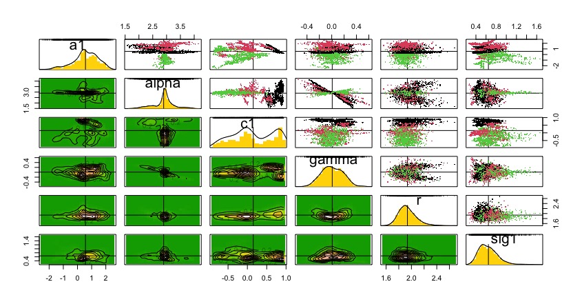
Although diagnostics for lambda.max decreases with more clones, the chains are not converging. It seems that this needs more iterations and change initial values.
Anyway, with these coefficients of the model, we can estimate latent count trajectories with the Kalman filter structure. This Kalman filter structure allows simultaneous estimation of latent states for observed time steps and prediction for missing ones, leveraging the temporal correlation in the process model.
Kalman.pred.acou.fn <- function() {
# Priors on model parameters: they are on the real line.
  parms ~ dmnorm(MuPost,PrecPost)
  a1 <- parms[1]
  alpha <- parms[2]   # intercept for scaling
  c1 <- parms[3]
  gamma <- parms[4]  # slope linking latent state X_t to mean
  r <- parms[5]      # overdispersion parameter for NegBinom
  sig1 <- parms[6]
  stovar1 <- 1/pow(sig1,2)

  # Likelihood
  mean_X1[1] <- a1/(1-c1) # Expected value of the first realization of the process
    # this is drawn from the stationary distribution of the process
    # Equation 14 (main text) and  A.4 in Appendix of Dennis et al 2006
    Varno1 <- pow(sig1,2)/(1-pow(c1,2)) #. Equation A.5 in Appendix of Dennis et al 2006

    # Updating the state: Stochastic process for all time steps
    X1[1]~dnorm(mean_X1[1], 1/Varno1); #first estimation of population
    log(lambda[1]) <- alpha + gamma * X1[1]
    C[1] <- log(lambda[1])
    #iteration of the GSS model in the data
    for (t in 2:qp1) {
      mean_X1[t] <- a1 + c1 * X1[(t - 1)]
      X1[t] ~ dnorm(mean_X1[t], stovar1) # Et is included here since a+cX(t-1) + Et ~ Normal(a+cX(t-1),sigma^2)

      Y1[(t-1)] ~ dnegbin(p[t], r)
      p[t] <- r/(r+lambda[t])
      log(lambda[t]) <- alpha + gamma * X1[t]
      C[t] <- log(lambda[t]) # expected count
    }
}
data4kalmanAco <- list(qp1 = as.numeric(length(final_df$acous_detections)),
Y1 = array(final_df$acous_detections,
dim = c(as.numeric(length(final_df$acous_detections)))),
MuPost = coef(dcrun.GSS.acou),
PrecPost = solve(vcov(dcrun.GSS.acou))) And run the Bayesian inference using the MLE from Data cloning
And we can generate a dataframe of the time series with the estimates, inter quartile range, and observed data through time
summary(BH_DC_Pred_Acou)
# extract predictions and CI around them
predAcou <- as.data.frame(t(mcmcapply(BH_DC_Pred_Acou, quantile, c(0.025, 0.5, 0.975))))


ExpectedCountsAcou <- as.data.frame(cbind(ExpectedCounts,predAcou))
# modify names
names(ExpectedCountsAcou) <- c("date","Time_w_alone","site_name","site_id",
                          "visit_number","common_name","time_window",
                          "Observed",
                          "AcousticDetections",
                          "DateTime","Time_window", "year",
                          "time_id",
                          "CountLower", "CountEstimated", "CountUpper",
                          "AcouDetLower", "AcouDetEstimated", "AcouDetUpper")

par(mar = c(5, 4, 7, 2))  # low, left, up, right

plot(x = ExpectedCountsAcou$DateTime,
     y = ExpectedCountsAcou$Observed,
     col = "#1b7837",
     ylim = c(0,40),
     ylab = "Counts",
     xlab = "Time (sampling window)")
points(x = ExpectedCountsAcou$DateTime,
     y = ExpectedCountsAcou$AcousticDetections,
     col = "#762a83")
lines(x = ExpectedCountsAcou$DateTime,
     y = ExpectedCountsAcou$CountEstimated,
     col = "#7fbf7b")
lines(x = ExpectedCountsAcou$DateTime,
     y = ExpectedCountsAcou$CountLower,
     col = "#d9f0d3", lty = 2)
lines(x = ExpectedCountsAcou$DateTime,
     y = ExpectedCountsAcou$CountUpper,
     col = "#d9f0d3", lty = 2)
lines(x = ExpectedCountsAcou$DateTime,
     y = ExpectedCountsAcou$AcouDetEstimated,
     col = "#af8dc3")
lines(x = ExpectedCountsAcou$DateTime,
     y = ExpectedCountsAcou$AcouDetLower,
     col = "#e7d4e8", lty = 2)
lines(x = ExpectedCountsAcou$DateTime,
     y = ExpectedCountsAcou$AcouDetUpper,
     col = "#e7d4e8", lty = 2)

legend(x = min(ExpectedCountsAcou$DateTime),
       y = 65,
       cex = 0.7,
       pt.cex = 0.7,
       xpd = TRUE,
       horiz = FALSE,
       legend = c("Observed from point counts",
                  "Acoustic detections",
                  "Estimate from point counts",
                  "Point count CI estimates",
                  "Estimate from acoustic detections",
                  "Acoustic detections CI estimates"),
       col = c("#1b7837",
               "#762a83",
               "#7fbf7b",
               "#d9f0d3",
               "#af8dc3",
               "#e7d4e8"),
       lty = c(NA, NA, 1, 2, 1, 2),   # NA for points, 1 for solid lines, 2 for dashed
       pch = c(1, 1, NA, NA, NA, NA), # symbols for points
       bty = "n")                     # no box around legend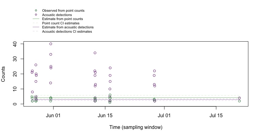
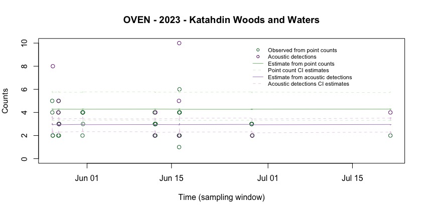
Cutting the edges to see the details of the estimates:
par(mar = c(6, 4, 4, 2))

plot(x = ExpectedCountsAcou$DateTime,
     y = ExpectedCountsAcou$Observed,
     col = "#1b7837",
     ylim = c(0,10),
     ylab = "Counts",
     xlab = "Time (sampling window)",
     main = "OVEN - 2023 - Katahdin Woods and Waters")
points(x = ExpectedCountsAcou$DateTime,
     y = ExpectedCountsAcou$AcousticDetections,
     col = "#762a83")
lines(x = ExpectedCountsAcou$DateTime,
     y = ExpectedCountsAcou$CountEstimated,
     col = "#7fbf7b")
lines(x = ExpectedCountsAcou$DateTime,
     y = ExpectedCountsAcou$CountLower,
     col = "#d9f0d3", lty = 2)
lines(x = ExpectedCountsAcou$DateTime,
     y = ExpectedCountsAcou$CountUpper,
     col = "#d9f0d3", lty = 2)
lines(x = ExpectedCountsAcou$DateTime,
     y = ExpectedCountsAcou$AcouDetEstimated,
     col = "#af8dc3")
lines(x = ExpectedCountsAcou$DateTime,
     y = ExpectedCountsAcou$AcouDetLower,
     col = "#e7d4e8", lty = 2)
lines(x = ExpectedCountsAcou$DateTime,
     y = ExpectedCountsAcou$AcouDetUpper,
     col = "#e7d4e8", lty = 2)

legend(x = quantile(ExpectedCountsAcou$DateTime, 0.75),
       y = 10,
       cex = 0.7,
       pt.cex = 0.7,
       xpd = TRUE,
       horiz = FALSE,
       legend = c("Observed from point counts",
                  "Acoustic detections",
                  "Estimate from point counts",
                  "Point count CI estimates",
                  "Estimate from acoustic detections",
                  "Acoustic detections CI estimates"),
       col = c("#1b7837",
               "#762a83",
               "#7fbf7b",
               "#d9f0d3",
               "#af8dc3",
               "#e7d4e8"),
       lty = c(NA, NA, 1, 2, 1, 2),   # NA for points, 1 for solid lines, 2 for dashed
       pch = c(1, 1, NA, NA, NA, NA), # symbols for points
       bty = "n")                     # no box around legend